CT
Jens Daniel Müller & Lara Burchardt
23 April, 2020
Last updated: 2020-04-23
Checks: 7 0
Knit directory: Baltic_Productivity/
This reproducible R Markdown analysis was created with workflowr (version 1.6.1). The Checks tab describes the reproducibility checks that were applied when the results were created. The Past versions tab lists the development history.
Great! Since the R Markdown file has been committed to the Git repository, you know the exact version of the code that produced these results.
Great job! The global environment was empty. Objects defined in the global environment can affect the analysis in your R Markdown file in unknown ways. For reproduciblity it’s best to always run the code in an empty environment.
The command set.seed(20191017) was run prior to running the code in the R Markdown file. Setting a seed ensures that any results that rely on randomness, e.g. subsampling or permutations, are reproducible.
Great job! Recording the operating system, R version, and package versions is critical for reproducibility.
Nice! There were no cached chunks for this analysis, so you can be confident that you successfully produced the results during this run.
Great job! Using relative paths to the files within your workflowr project makes it easier to run your code on other machines.
Great! You are using Git for version control. Tracking code development and connecting the code version to the results is critical for reproducibility.
The results in this page were generated with repository version 8c4ccb4. See the Past versions tab to see a history of the changes made to the R Markdown and HTML files.
Note that you need to be careful to ensure that all relevant files for the analysis have been committed to Git prior to generating the results (you can use wflow_publish or wflow_git_commit). workflowr only checks the R Markdown file, but you know if there are other scripts or data files that it depends on. Below is the status of the Git repository when the results were generated:
Ignored files:
    Ignored:    .Rhistory
    Ignored:    .Rproj.user/
    Ignored:    data/ARGO/
    Ignored:    data/Finnmaid/
    Ignored:    data/GETM/
    Ignored:    data/OSTIA/
    Ignored:    data/_merged_data_files/
    Ignored:    data/_summarized_data_files/
Note that any generated files, e.g. HTML, png, CSS, etc., are not included in this status report because it is ok for generated content to have uncommitted changes.
These are the previous versions of the repository in which changes were made to the R Markdown (analysis/CT.Rmd) and HTML (docs/CT.html) files. If you’ve configured a remote Git repository (see ?wflow_git_remote), click on the hyperlinks in the table below to view the files as they were in that past version.
| File | Version | Author | Date | Message |
|---|---|---|---|---|
| Rmd | 8c4ccb4 | LSBurchardt | 2020-04-23 | #3 functionality largely improved |
| html | 84b3027 | jens-daniel-mueller | 2020-04-23 | Build site. |
| Rmd | b54b53b | jens-daniel-mueller | 2020-04-23 | deleted wrong legend name (ppp) in deployment plot |
| html | b11301c | jens-daniel-mueller | 2020-04-22 | Build site. |
| Rmd | 30999c4 | jens-daniel-mueller | 2020-04-22 | used ppp_2 in SST time series plots |
| html | 940357e | jens-daniel-mueller | 2020-04-22 | Build site. |
| Rmd | 0b5a17a | LSBurchardt | 2020-04-21 | #3 ++ lot of the issues solved: |
| html | 0055ce4 | jens-daniel-mueller | 2020-04-17 | Build site. |
| Rmd | dfdabc7 | jens-daniel-mueller | 2020-04-17 | correct NA data in plots |
| html | 90ced1b | jens-daniel-mueller | 2020-04-17 | Build site. |
| Rmd | 8ecbd8f | jens-daniel-mueller | 2020-04-17 | separate chunks for criteria, criteria named in plain text, new headers |
| html | ecb4f87 | jens-daniel-mueller | 2020-04-17 | Build site. |
| Rmd | f2a95e8 | jens-daniel-mueller | 2020-04-17 | CT y_axis grid 20 |
| html | f0231f7 | jens-daniel-mueller | 2020-04-17 | Build site. |
| Rmd | e801aae | jens-daniel-mueller | 2020-04-17 | figure aspect ratio and uniform color scales |
| html | c9c143e | jens-daniel-mueller | 2020-04-17 | Build site. |
| Rmd | 5528d3d | jens-daniel-mueller | 2020-04-17 | knit: corrected PPP assignment, revised plots |
| Rmd | 160c8f8 | LSBurchardt | 2020-04-17 | #3 reliable enumeration of ppp with individual control variable |
| html | a780d69 | jens-daniel-mueller | 2020-04-17 | Build site. |
| Rmd | 7507a93 | jens-daniel-mueller | 2020-04-17 | PPP labeling with 4 day gap |
| Rmd | 8ea672d | LSBurchardt | 2020-04-16 | #3 end criterion corrected, ppps colored per year |
| Rmd | 33a1b74 | LSBurchardt | 2020-04-16 | #3 commented, prevented from getting rm() warning |
| html | e62e49c | jens-daniel-mueller | 2020-04-16 | Build site. |
| Rmd | 5340b36 | jens-daniel-mueller | 2020-04-16 | revised PPP indentification, added SST plot; referring to l. 581: Warning messages: 1: In rm(start, roll_index_df, roll_index, roll_value, |
| Rmd | 6ba4e29 | LSBurchardt | 2020-04-15 | #3 multiple problems with ppp identification solved: enumeration working, end_criteria only kick in when there was a start, duplicates deleted, minimum CT within 7 day forward is used as identifier for ppp |
| html | 8737000 | jens-daniel-mueller | 2020-04-15 | Build site. |
| Rmd | 5488726 | jens-daniel-mueller | 2020-04-15 | minor aesthetic changes before re-knitting |
| html | a1a3e25 | jens-daniel-mueller | 2020-04-15 | Build site. |
| Rmd | 9cc640c | jens-daniel-mueller | 2020-04-15 | minor aesthetic changes before re-knitting |
| html | be8517f | jens-daniel-mueller | 2020-04-15 | Build site. |
| Rmd | 170667e | jens-daniel-mueller | 2020-04-15 | added plots for PPP |
| Rmd | 01a1f1b | LSBurchardt | 2020-04-14 | var_all unified to names(nc$var) |
| Rmd | 18ca5af | LSBurchardt | 2020-04-14 | #3 ppp ident updated, saving works, enumeration still ongoing |
| html | c4a1b00 | jens-daniel-mueller | 2020-04-14 | Build site. |
| Rmd | 19eeda2 | jens-daniel-mueller | 2020-04-14 | correct NGS limits, all csv files recreated, PPP identification started |
| Rmd | a165baa | LSBurchardt | 2020-04-14 | #3 ppp identificiation: problems when no ppp is found, then if function returns error; saving not finished yet, currrently df_ppp_temp is overwritten every loop –> exist function missing, will be added shortly |
| Rmd | ac9cad0 | LSBurchardt | 2020-04-09 | vroom to write_/read_csv; as.data.frame to as_tibble; tidyverse piping |
| Rmd | d00d732 | jens-daniel-mueller | 2020-04-08 | formatting header # corrected, not knitted yet |
| html | 6f29d15 | jens-daniel-mueller | 2020-04-08 | Build site. |
| Rmd | f33624a | jens-daniel-mueller | 2020-04-08 | knitted with deployment detection |
| Rmd | bf0b055 | LSBurchardt | 2020-04-07 | #3 vroom to write.csv/read_csv; theoretically ready to knit |
| Rmd | abc2d8d | LSBurchardt | 2020-04-07 | #3 deployment values implemented, plotted |
| Rmd | 6907a02 | LSBurchardt | 2020-04-07 | NGS limits changed to: 58.5-59.0 in all files; pivot-wider problem solved in CT.Rmd |
| html | a98bf60 | jens-daniel-mueller | 2020-04-06 | Build site. |
| Rmd | 5d352db | jens-daniel-mueller | 2020-04-06 | calculated CT in equilibrium with atmosphere and updated CT dygraph |
| Rmd | 662c74a | jens-daniel-mueller | 2020-04-03 | added explanatory comments |
| Rmd | c619811 | LSBurchardt | 2020-04-03 | #3 comments |
| html | a4ab61e | jens-daniel-mueller | 2020-03-31 | Build site. |
| Rmd | 1518256 | jens-daniel-mueller | 2020-03-31 | updated dygraphs |
| html | 67a6e2b | jens-daniel-mueller | 2020-03-31 | Build site. |
| Rmd | 5e275d2 | jens-daniel-mueller | 2020-03-31 | CT and flux calculation included |
| Rmd | ef65647 | LSBurchardt | 2020-03-31 | #3 flux calculations and graphs prepared, calculations are not running on my PC though |
| Rmd | 3f94314 | LSBurchardt | 2020-03-27 | #3 windspeed extraction working |
| Rmd | 2ca3f71 | LSBurchardt | 2020-03-23 | #3 extracting S,T, pco2 for all routes; windspeed from GETM with problem |
| html | abc5f7d | jens-daniel-mueller | 2020-03-18 | Build site. |
| Rmd | 10176c9 | jens-daniel-mueller | 2020-03-18 | knit after Lara updated CT |
| html | b80d3a6 | jens-daniel-mueller | 2020-03-18 | Build site. |
| Rmd | 8023757 | jens-daniel-mueller | 2020-03-18 | knit after Lara updated CT |
| Rmd | 03ea2de | LSBurchardt | 2020-03-18 | #1 ready to knit to html: CT with Plot, probably little more explanatory background needed for webside |
| html | 03646b4 | jens-daniel-mueller | 2020-03-16 | Build site. |
| html | 6394f58 | jens-daniel-mueller | 2020-03-16 | Build site. |
| Rmd | 9b0eb49 | LSBurchardt | 2020-03-15 | #1 ready to knit html: SSS working, CT, MLD_pCO2 and SST updated to new data |
| html | e1acb2d | jens-daniel-mueller | 2020-03-09 | Build site. |
| html | c15b71c | jens-daniel-mueller | 2020-03-09 | Build site. |
| Rmd | 9332cae | jens-daniel-mueller | 2020-03-09 | restructered content into chapters, rebuild site, except SSS |
| Rmd | fa8ef89 | Burchardt | 2020-02-28 | #1 new CT.rmd and sss.rmd |
| Rmd | 1663eee | Burchardt | 2020-02-13 | #1 CT new |
library(tidyverse)
library(ncdf4)
library(vroom)
library(lubridate)
library(geosphere)
library(dygraphs)
library(xts)
library(here)
library(seacarb)
library(zoo)
# route
select_route <- c("E", "F", "G", "W", "X")
# variable names in 2d and 3d GETM files
var <- "SSS_east"
# latitude limits
low_lat <- 58.5
high_lat <- 59.01 Regional mean salinity
The mean salinity was calculated across all measurments made between march - september in the NGS subregion.
nc <- nc_open(paste("data/Finnmaid/", "FM_all_2019_on_standard_tracks.nc", sep = ""))

# read required vectors from netcdf file
route <- ncvar_get(nc, "route")
route <- unlist(strsplit(route, ""))
date_time <- ncvar_get(nc, "time")
latitude_east <- ncvar_get(nc, "latitude_east")

array <- ncvar_get(nc, var) # store the data in a 2-dimensional array
#dim(array) # should have 2 dimensions: 544 coordinate, 2089 time steps

  fillvalue <- ncatt_get(nc, var, "_FillValue")
  array[array == fillvalue$value] <- NA
  rm(fillvalue)

  #i <- 5
  for (i in seq(1,length(route),1)){


    if(route[i] %in% select_route) {
      slice <- array[i,]

      value <- mean(slice[latitude_east > low_lat & latitude_east < high_lat], na.rm = TRUE)
      sd    <- sd(slice[latitude_east > low_lat & latitude_east < high_lat], na.rm = TRUE)
      date <- ymd("2000-01-01") + date_time[i]

      temp <- bind_cols(date = date, var=var, value = value, sd = sd)

      if (exists("timeseries", inherits = FALSE)){
        timeseries <- bind_rows(timeseries, temp)
      } else{timeseries <- temp}

      rm(temp, value, date, sd)

    }
  }
nc_close(nc)

fm_sss__ngs <- timeseries %>%
  mutate(sss = value,
         year = year(date),
         month = month(date))

fm_sss_ngs_monthlymean <- fm_sss__ngs %>%
  filter(month >=3 , month <=9) %>%
  summarise(sss_mean = mean(sss, na.rm = TRUE))


rm(array,fm_sss__ngs,nc, timeseries, date_time,
  i, latitude_east, route, slice, var)
The mean salinity between March and September for the NGS subregion for all years is 6.56.
2 Finnmaid data extraction
pCO2 and SST observations in NGS were extracted for all crossings.
nc <- nc_open(paste("data/Finnmaid/", "FM_all_2019_on_standard_tracks.nc", sep = ""))

#names(nc$var) # uncomment to print variable names and select relevant index
index <- c(9,11) #index of wanted variables SST_east and pCO2 east
var_all <- c(names(nc$var[index]))

# read required vectors from netcdf file
route <- ncvar_get(nc, "route")
route <- unlist(strsplit(route, ""))
date_time <- ncvar_get(nc, "time")
latitude_east <- ncvar_get(nc, "latitude_east")

for (var in var_all) {

  #print(var)

  array <- ncvar_get(nc, var) # store the data in a 2-dimensional array
  #dim(array) # should have 2 dimensions: 544 coordinate, 2089 time steps

  fillvalue <- ncatt_get(nc, var, "_FillValue")
  array[array == fillvalue$value] <- NA
  rm(fillvalue)

    for (i in seq(1,length(route),1)){


    if(route[i] %in% select_route) {
      slice <- array[i,]

      value <- mean(slice[latitude_east > low_lat & latitude_east < high_lat], na.rm = TRUE)
      sd    <- sd(slice[latitude_east > low_lat & latitude_east < high_lat], na.rm = TRUE)
      date <- ymd("2000-01-01") + date_time[i]

      fm_ngs_all_routes_part <- bind_cols(date = date, var=var, value = value, sd = sd, route=route[i])

      if (exists("fm_ngs_all_routes", inherits = FALSE)){
        fm_ngs_all_routes <- bind_rows(fm_ngs_all_routes, fm_ngs_all_routes_part)
      } else{fm_ngs_all_routes <- fm_ngs_all_routes_part}

      rm(fm_ngs_all_routes_part, value, date, sd, slice)

      }
    }
  rm(array, var,i)
}

nc_close(nc)

fm_ngs_all_routes %>%
  write_csv(here::here("data/_summarized_data_files/", file = "fm_ngs_all_routes.csv"))

rm(nc, fm_ngs_all_routes, latitude_east, route,date_time)
3 GETM windspeed
Reanalysis windspeed data as used in the GETM model run were used.
filesList_2d <- list.files(path= "data", pattern = "Finnmaid.E.2d.20", recursive = TRUE)

file <- filesList_2d[1]
nc <- nc_open(paste("data/", file, sep = ""))

names(nc$var)
index <- c(11,12) # index of wanted variables u10 and v10
var_all <- c(names(nc$var[index]))


lon <- ncvar_get(nc, "lonc")
lat <- ncvar_get(nc, "latc", verbose = F)
nc_close(nc)

rm(file, nc)

for (var in var_all){

for (n in 1:length(filesList_2d)) {

file <- filesList_2d[n]

nc <- nc_open(paste("data/", file, sep = ""))

time_units <- nc$dim$time$units %>%     #we read the time unit from the netcdf file to calibrate the time
    substr(start = 15, stop = 33) %>%   #calculation, we take the relevant information from the string
    ymd_hms()                           # and transform it to the right format

t <- time_units + ncvar_get(nc, "time")

array <- ncvar_get(nc, var) # store the data in a 2-dimensional array
dim(array) # should be 2d with dimensions: 544 coordinate, 31d*(24h/d/3h)=248 time steps

array <- as.data.frame(t(array), xy=TRUE)
array <- as_tibble(array)

gt_windspeed_ngs_part <- array %>%
  set_names(as.character(lat)) %>%
  mutate(date_time = t) %>%
  gather("lat", "value", 1:length(lat)) %>%
  mutate(lat = as.numeric(lat)) %>%
  filter(lat > low_lat, lat<high_lat) %>%
  group_by(date_time) %>%
  summarise_all("mean") %>%
  ungroup() %>%
  mutate(var = var)


if (exists("gt_windspeed_ngs")) {gt_windspeed_ngs <- bind_rows(gt_windspeed_ngs, gt_windspeed_ngs_part)
  }else {gt_windspeed_ngs <- gt_windspeed_ngs_part}

  nc_close(nc)
  rm(array, nc, t, gt_windspeed_ngs_part)
  print(n) # to see working progress
}

print(paste("gt_", var, "_ngs.csv", sep = "")) # to see working progress


rm(n, file, time_units)
}

rm(filesList_2d, var, var_all, lat, lon)


gt_windspeed_ngs <- gt_windspeed_ngs %>%
  group_by(date_time, var) %>%
  summarise(mean_value= mean(value)) %>%
  pivot_wider(values_from = mean_value, names_from = var) %>%
  mutate(U_10 = round(sqrt(u10^2 + v10^2), 3)) %>%
  select(-c(u10, v10))

gt_windspeed_ngs %>%
  write_csv(here::here("data/_summarized_data_files/", file = paste("gt_windspeed_ngs.csv")))

rm(gt_windspeed_ngs)
4 CT calculation
CT was calculated from measured pCO2 based on a fixed mean alkalinity value of 1650 µmol kg-1.
df <- read_csv(here::here("data/_summarized_data_files/", file =  "fm_ngs_all_routes.csv"))

df <- df %>%
  select(date, var, value, route)

df <- df %>%
  # drop_na() %>%
  pivot_wider(values_from = value, names_from = var) %>%
  drop_na()

#calculation of CT based on pCO2 (var1) and alkalinity (var2) as input parameters
#calculation of CT in theoretical equilibrium with atmosphere (CT_equi) based on pCO2_air (var1) and alkalinity (var2) as input parameters

df <- df %>%
  rename(SST = SST_east,
         pCO2 = pCO2_east) %>%
  #drop_na() %>%
  mutate(CT = carb(24,
                   var1=pCO2,
                   var2=1650*1e-6,
                   S=pull(fm_sss_ngs_monthlymean),
                   T=SST,
                   k1k2="m10", kf="dg", ks="d", gas="insitu")[,16]*1e6) %>%
  mutate(year = year(date),
         pCO2_air = 400 - 2*(2015-year),
         CT_equi = carb(24,
                   var1=pCO2_air,
                   var2=1650*1e-6,
                   S=pull(fm_sss_ngs_monthlymean),
                   T=SST,
                   k1k2="m10", kf="dg", ks="d", gas="insitu")[,16]*1e6) %>%
  select(-c(pCO2_air, year))


df %>%
   write_csv(here::here("data/_summarized_data_files/", file = "fm_CT_ngs.csv"))

rm(df)
5 Air-sea CO2 flux
The CO2 flux across the sea surface was calculated according to Wanninkhof (2014).
df_1 <- read_csv(here::here("data/_summarized_data_files/", file = "fm_CT_ngs.csv"))
df_2 <- read_csv(here::here("data/_summarized_data_files/", file = "gt_windspeed_ngs.csv"))

df_2 <- df_2 %>%
  mutate(date = as.Date(date_time)) %>%
  select(date, U_10) %>%
  group_by(date) %>%
  summarise_all("mean") %>%
  ungroup()

df <- full_join(df_1, df_2, by = "date") %>%
  arrange(date)

rm(df_1,df_2)

df <- df %>%
  mutate(year = year(date),
         pCO2_int = na.approx(pCO2, na.rm = FALSE),                  #na.approx: replacing NA with interpolated values
         SST_int = na.approx(SST, na.rm = FALSE)) %>%
  filter(!is.na(pCO2_int))

#Calculation of the Schmidt number as a funktion of temperature according to Wanninkhof (2014)
Sc_W14 <- function(tem) {
  2116.8 - 136.25 * tem + 4.7353 * tem^2 - 0.092307 * tem^3 + 0.0007555 * tem^4
}

Sc_W14(20)

# calculate flux F [mol m–2 d–1]
df <- df %>%
  mutate(pCO2_air = 400 - 2*(2015-year),
         dpCO2 = pCO2_int - pCO2_air,
         dCO2  = dpCO2 * K0(S=pull(fm_sss_ngs_monthlymean), T=SST_int),
         k     = 0.251 * U_10^2 * (Sc_W14(SST_int)/660)^(-0.5),
         flux_daily = k*dCO2*1e-5*24)


df %>%
   write_csv(here::here("data/_merged_data_files/", file = paste("gt_fm_flux_ngs.csv")))

rm(df, Sc_W14)
6 Time series CT, MLD, SST, windspeed, and air-sea fluxes
# read CT and flux data
gt_fm_flux_ngs <- read_csv(here::here("data/_merged_data_files/", file = "gt_fm_flux_ngs.csv"))

gt_fm_flux_ngs <- gt_fm_flux_ngs %>%
  mutate(date = as.Date(date))

ts_xts_CT <- xts(cbind(gt_fm_flux_ngs$CT, gt_fm_flux_ngs$CT_equi), order.by = gt_fm_flux_ngs$date)
names(ts_xts_CT) <- c("CT", "CT_equi")

ts_xts_SST <- xts(gt_fm_flux_ngs$SST, order.by = gt_fm_flux_ngs$date)
names(ts_xts_SST) <- "SST"

ts_xts_windspeed <- xts(gt_fm_flux_ngs$U_10, order.by = gt_fm_flux_ngs$date)
names(ts_xts_windspeed) <- "Windspeed"

ts_xts_flux <- xts(gt_fm_flux_ngs$flux_daily, order.by = gt_fm_flux_ngs$date)
names(ts_xts_flux) <- "Daily Flux"


# read MLD data
gt_mld_fm_pco2_ngs <-
  read_csv(here::here("data/_merged_data_files/", file = "gt_mld_fm_pco2_ngs.csv"))

gt_mld_fm_pco2_ngs <- gt_mld_fm_pco2_ngs %>%
  mutate(date = as.Date(date))

ts_xts_mld5 <- xts(gt_mld_fm_pco2_ngs$value_mld5, order.by = gt_mld_fm_pco2_ngs$date)
names(ts_xts_mld5) <- "mld_age_5"

ts_xts_CT %>%
  dygraph(group = "Fluxes") %>%
  dyRangeSelector(dateWindow = c("2014-01-01", "2016-12-31")) %>%
  dySeries("CT") %>%
  dyAxis("y", label = "CT") %>%
  dyOptions(drawPoints = TRUE, pointSize = 1.5, connectSeparatedPoints=TRUE, strokeWidth=0.5,
            drawAxesAtZero=TRUE)
ts_xts_SST %>%
dygraph(group = "Fluxes") %>%
dyRangeSelector(dateWindow = c("2014-01-01", "2016-12-31")) %>%
dySeries("SST") %>%
dyAxis("y", label = "SST") %>%
dyOptions(drawPoints = TRUE, pointSize = 1.5, connectSeparatedPoints=TRUE, strokeWidth=0.5,
drawAxesAtZero=TRUE)ts_xts_mld5 %>%
dygraph(group = "Fluxes") %>%
dyRangeSelector(dateWindow = c("2014-01-01", "2016-12-31")) %>%
dySeries("mld_age_5") %>%
dyAxis("y", label = "mld_age_5") %>%
dyOptions(drawPoints = TRUE, pointSize = 1.5, connectSeparatedPoints=TRUE, strokeWidth=0.5,
drawAxesAtZero=TRUE)ts_xts_windspeed %>%
dygraph(group = "Fluxes") %>%
dyRangeSelector(dateWindow = c("2014-01-01", "2016-12-31")) %>%
dySeries("Windspeed") %>%
dyAxis("y", label = "Windspeed [m/s]") %>%
dyOptions(drawPoints = TRUE, pointSize = 1.5, connectSeparatedPoints=TRUE, strokeWidth=0.5,
drawAxesAtZero=TRUE)ts_xts_flux %>%
dygraph(group = "Fluxes") %>%
dyRangeSelector(dateWindow = c("2014-01-01", "2016-12-31")) %>%
dySeries("Daily Flux") %>%
dyAxis("y", label = "Daily Flux") %>%
dyOptions(drawPoints = TRUE, pointSize = 1.5, connectSeparatedPoints=TRUE, strokeWidth=0.5)rm(gt_fm_flux_ngs, gt_mld_fm_pco2_ngs,
ts_xts_CT, ts_xts_flux, ts_xts_mld5, ts_xts_SST, ts_xts_windspeed)7 Identification of continous deployment periods
# time

time_low <- 03 # 03 as month March
time_high <- 09 # 09 as month September

deployment_gap <- 7- The maximum allowed gap was defined as 7 day.
df <-
   read_csv(here::here("data/_summarized_data_files/", file = "fm_CT_ngs.csv"))

df <- df %>%
  mutate (month = month(date),
          year = year(date)) %>%
  filter (month >= time_low & month <= time_high) %>%
  group_by(year) %>%
  mutate(deployment =
           as.factor(cumsum(c(TRUE,diff(date)>= deployment_gap)))) %>% # deployment +1, when data gap > 7 days
  ungroup()

df %>%
  ggplot(aes( x = as.Date(yday(date)), y = year, color = deployment))+
  geom_point()+
  scale_y_reverse(breaks = seq(2000,2030,1))+
  scale_x_date(date_minor_breaks = "week",
               date_labels = "%b")+
  scale_color_brewer(palette = "Set1")+
  theme(axis.title.x = element_blank())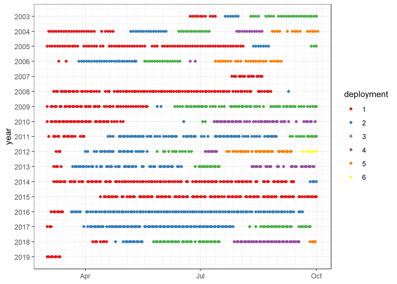
df %>%
  write_csv(here::here("data/_summarized_data_files/", file="fm_CT_ngs_deployments.csv"))
8 Identification of primary production periods (PPP)
#criteria
decrease_start <- 20
timespan_start <- 7 #in days

decrease_end <- 20
timespan_end <- 7 #in days
The following criteria are implemented in the following to find periods of primary production:
- CT is lower than at equilibrium with the atmosphere
- period must be within one deployment
- starts at a day followed by 7 days in which CT decreased at least by 20
- ends at day where the CT drop was below 20 for the previous 7
PPPs are numbered.
# databasis

df <-
   read_csv(here::here("data/_summarized_data_files/", file = "fm_CT_ngs_deployments.csv"))

# identification

#ppp identified per year, per deployment, only when CT < CT_equi


df_ppp <- df %>%
  filter(CT < CT_equi)

years <- (unique(df_ppp$year))

# first of three loops, loops through each observatio year
# we get the number of deployments within this year for further analysis
for (n in years) {

  a <- 1

  deployment_year <- df_ppp %>%
    filter(year == n)

  deployment_values <- unique(deployment_year$deployment)

  start <- "stop"
  end <- "stop"

  # second of three loops, loops through each deployment within on year
  for (d in deployment_values){

    a <- a+1

    df_ppp_temp <- df_ppp %>%
      filter(year == n  , deployment == d) %>%
      mutate(ppp = NA)

    # third of three loops, within on deployment of year n, we check ppp criteria for every row
    for (x in 1:nrow(df_ppp_temp)){

    if (start == "stop" & end == "stop" & is.na(df_ppp_temp$ppp[x]) == TRUE){a <- a +1
    } else {a <- a}

    ##start criteria
    # define subdataset looking forward "timespan_start" days
    lag_start <- df_ppp_temp %>%
    filter(date >= date[x], date <= (date[x]+ duration(timespan_start, 'days')))

    roll_index <- which.min(lag_start$CT)  #Minimum CT-value in 7 day forward
    roll_value <- lag_start$CT[roll_index] # get exact minimum CT value within subdataset

    # we only proceed, if there is a minimum CT value
    if (is_empty(roll_value)== FALSE){

    # get index of exact CT value in whole dataset
    roll_index_df <- df_ppp_temp %>%
    mutate(row_no = row_number()) %>%
    filter(CT == roll_value) %>%
    select(row_no) %>%
    as.numeric()

    # second if-condition for start criteria; is CT value of current loop date x more than "decrease_start" higher tha minimum CT in 7 day forward

    if (df_ppp_temp$CT[x]-roll_value >= decrease_start) {

    start <- "go" #condition for end-criteria; only TRUE when there was the necessary decrease

    df_ppp_temp$ppp[x:roll_index_df] <- as.numeric(a)

    } else{start <- "stop"} # end of l. 566; if CT >= decrease_start

    rm(roll_index_df)

    } else {} # end of l.555 ;if we don't have a roll_value or the criterion of decrease is not met start is set FALSE, so that end criteria don't kick in without a start


    ##end criteria

    #was there a start?
    if (start == "go" | start == "stop" & end == "go"| start == "go" & end == "go"){

    lag_end <- df_ppp_temp %>%
    filter(date < date[x], date >= (date[x]- duration(timespan_end, 'days')))

    roll_index <- which.max(lag_end$CT) #in contrast to start we search for the maximum CT value here when looking backwards
    roll_value <- lag_end$CT[roll_index]

    if (is_empty(roll_value) == FALSE){ #at the start of the loop we can't look backwards

    roll_index_df <- df_ppp_temp %>%
    mutate(row_no = row_number()) %>%
    filter(CT == roll_value) %>%
    select(row_no) %>%
    as.numeric()

    if (roll_value-df_ppp_temp$CT[x] >= decrease_end){

    df_ppp_temp$ppp[x] = as.numeric(a)
    end <- "go"

    rm(roll_index_df)

    } else{end <- "stop"} # end of l.598; if CT >= decrease_end

    } else {}             # end of l.590; if roll_value = empty; if we can't look backwards, we jump to the next loop iteration

    rm(lag_end)

    } else {end <- "stop"
      start < "stop"}   #end l. 582; start == TRUE condition

    rm(roll_index, roll_value)

    } #end  loop through df_ppp_temp

    if (exists("fm_ppp", inherits = FALSE)){
        fm_ppp <- bind_rows(fm_ppp, df_ppp_temp)
    }else{fm_ppp <- df_ppp_temp}

    rm(df_ppp_temp)

  }#end of loop through deployments

  rm(deployment_year, deployment_values)

}#end of loop through years


fm_ppp_na <- fm_ppp %>%
  drop_na()

# enumeration of ppps

#ppps continous numerations
fm_ppp_final <- fm_ppp_na %>%
  group_by(year) %>%
  mutate(ppp_2 = as.factor(cumsum(c(TRUE,abs(diff(ppp))>=1)))) %>%
  ungroup()

ggplot()+
  geom_point(data = df, aes(as.Date(yday(date)), year), col="grey")+
  geom_point(data = fm_ppp_final, aes(as.Date(yday(date)), year, col = as.factor(ppp_2)))+
  scale_y_reverse(breaks = seq(2000,2030,1))+
  scale_x_date(date_minor_breaks = "week",
               date_labels = "%b")+
  scale_color_brewer(palette = "Set1", name="PPP")+
  theme(axis.title.x = element_blank())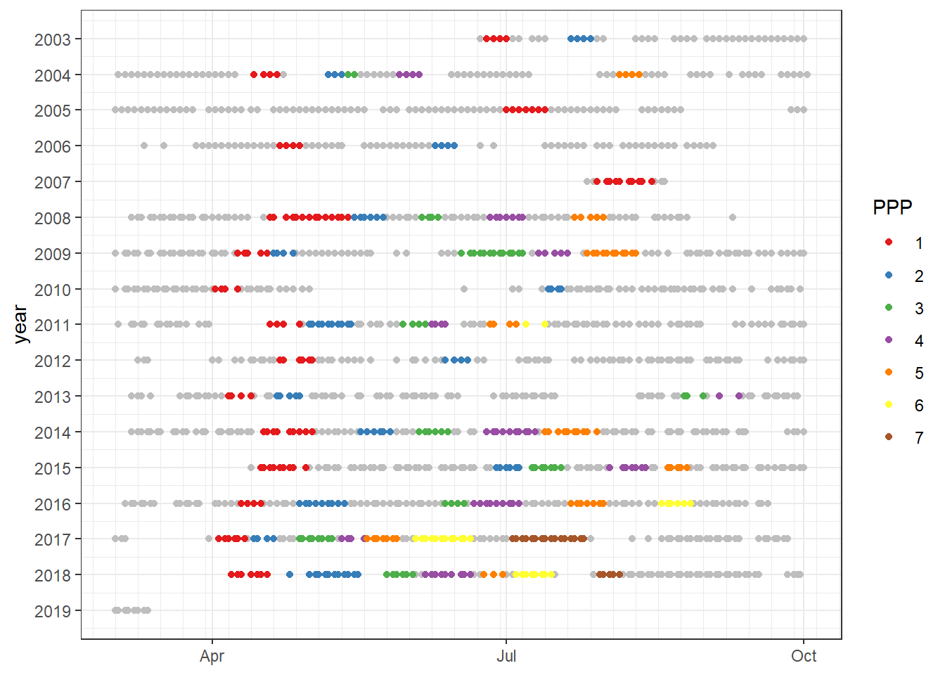
fm_ppp_final %>%
  write_csv(here::here("data/_summarized_data_files/", file = "fm_ppp_ngs.csv"))
8.1 CT yearly time series
ggplot()+
  geom_point(data = df, aes(as.Date(yday(date)), CT), color = "grey")+
  geom_point(data = fm_ppp_final, aes(as.Date(yday(date)), CT, color = as.factor(ppp_2)))+
  scale_y_continuous(breaks = seq(1000,2000,100),
                     minor_breaks = seq(1000,2000,20))+
  scale_x_date(date_minor_breaks = "week",
               date_labels = "%b")+
  scale_color_brewer(palette = "Set1", name="PPP")+
  theme(axis.title.x = element_blank(),
        legend.position = "bottom")+
  facet_grid(year~.)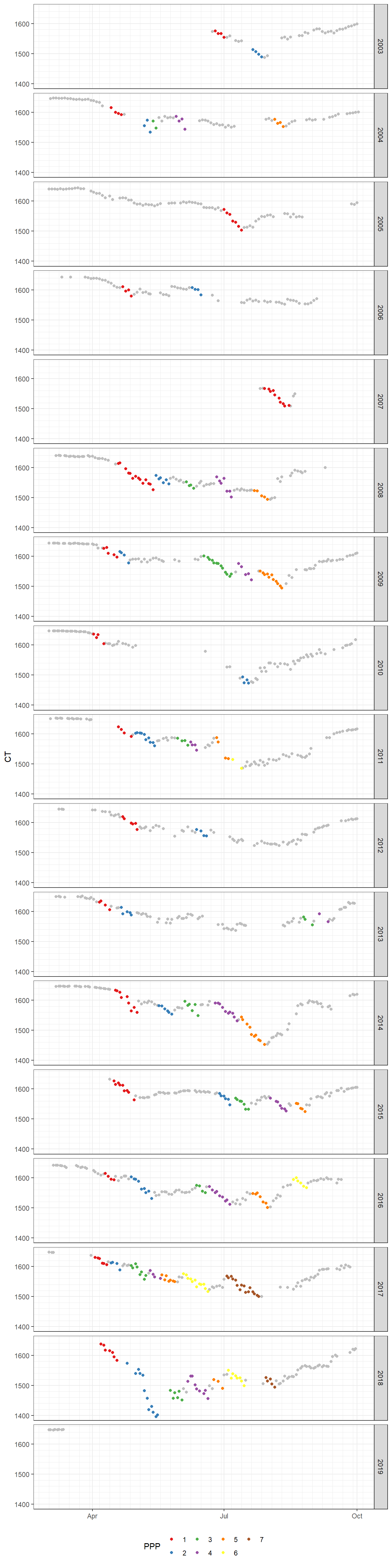
8.2 SST yearly time series
ggplot()+
  geom_point(data = df, aes(as.Date(yday(date)), SST), color = "grey")+
  geom_point(data = fm_ppp_final, aes(as.Date(yday(date)), SST, color = as.factor(ppp_2)))+
  scale_x_date(date_minor_breaks = "week",
               date_labels = "%b")+
  scale_color_brewer(palette = "Set1", name="PPP")+
  theme(axis.title.x = element_blank(),
        legend.position = "bottom")+
  facet_grid(year~.)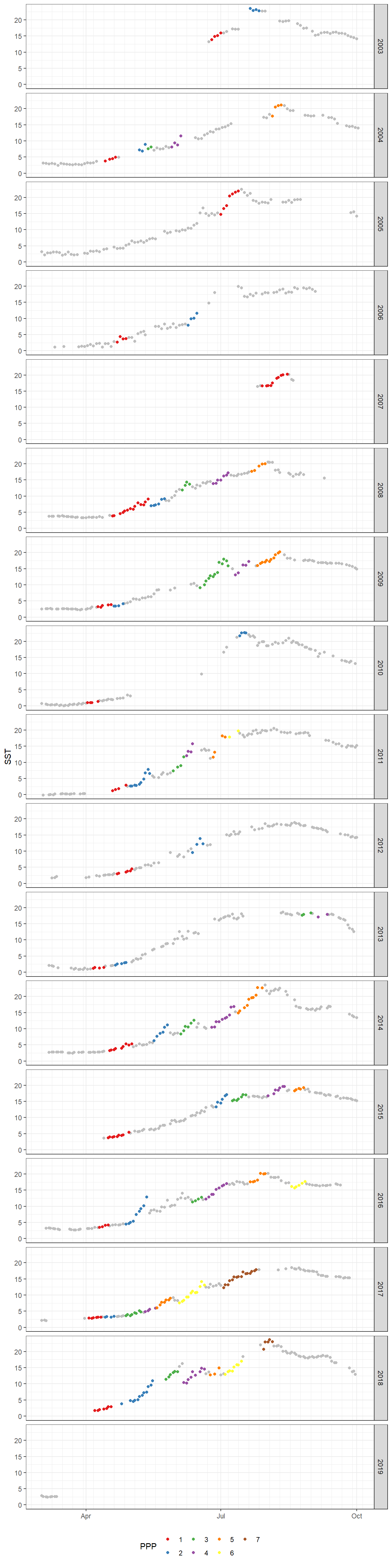
9 Tasks / open questions
- check drop_na() before CT calculation, because thise removes quite a lot data points where only SST is missing.
- drop_na() before pivot_wider: leaves 2016 observations
- drop_na() after pivot_wider or second drop_na() just before CT calculations: leaves 1982 observations, we loose timeperiods without SST value from: “2005-8-25” to “2005-9-24” and “2006-01-29” to “2006-03-04”
- still we need to keep drop_na() after pivot_wider for now, because CT calculation does not accept NA data in any column
sessionInfo()R version 3.6.3 (2020-02-29)
Platform: i386-w64-mingw32/i386 (32-bit)
Running under: Windows 10 x64 (build 18363)
Matrix products: default
locale:
[1] LC_COLLATE=English_Germany.1252 LC_CTYPE=English_Germany.1252
[3] LC_MONETARY=English_Germany.1252 LC_NUMERIC=C
[5] LC_TIME=English_Germany.1252
attached base packages:
[1] stats graphics grDevices utils datasets methods base
other attached packages:
[1] seacarb_3.2.13 oce_1.2-0 gsw_1.0-5 testthat_2.3.2
[5] here_0.1 xts_0.12-0 zoo_1.8-7 dygraphs_1.1.1.6
[9] geosphere_1.5-10 lubridate_1.7.4 vroom_1.2.0 ncdf4_1.17
[13] forcats_0.5.0 stringr_1.4.0 dplyr_0.8.5 purrr_0.3.3
[17] readr_1.3.1 tidyr_1.0.2 tibble_3.0.0 ggplot2_3.3.0
[21] tidyverse_1.3.0 workflowr_1.6.1
loaded via a namespace (and not attached):
[1] Rcpp_1.0.4 whisker_0.4 knitr_1.28 xml2_1.3.0
[5] magrittr_1.5 hms_0.5.3 rvest_0.3.5 tidyselect_1.0.0
[9] bit_1.1-15.2 colorspace_1.4-1 lattice_0.20-41 R6_2.4.1
[13] rlang_0.4.5 fansi_0.4.1 broom_0.5.5 xfun_0.12
[17] dbplyr_1.4.2 modelr_0.1.6 withr_2.1.2 git2r_0.26.1
[21] ellipsis_0.3.0 htmltools_0.4.0 assertthat_0.2.1 bit64_0.9-7
[25] rprojroot_1.3-2 digest_0.6.25 lifecycle_0.2.0 haven_2.2.0
[29] rmarkdown_2.1 sp_1.4-1 compiler_3.6.3 cellranger_1.1.0
[33] pillar_1.4.3 scales_1.1.0 backports_1.1.5 generics_0.0.2
[37] jsonlite_1.6.1 httpuv_1.5.2 pkgconfig_2.0.3 rstudioapi_0.11
[41] munsell_0.5.0 httr_1.4.1 tools_3.6.3 grid_3.6.3
[45] nlme_3.1-145 gtable_0.3.0 utf8_1.1.4 DBI_1.1.0
[49] cli_2.0.2 readxl_1.3.1 yaml_2.2.1 crayon_1.3.4
[53] farver_2.0.3 RColorBrewer_1.1-2 later_1.0.0 promises_1.1.0
[57] htmlwidgets_1.5.1 fs_1.4.0 vctrs_0.2.4 glue_1.3.2
[61] evaluate_0.14 labeling_0.3 reprex_0.3.0 stringi_1.4.6