SST

workflowr

• Summary
• Checks
• Past versions

Last updated: 2020-04-14

Checks: 7 0

Knit directory: Baltic_Productivity/

This reproducible R Markdown analysis was created with workflowr (version 1.6.1). The Checks tab describes the reproducibility checks that were applied when the results were created. The Past versions tab lists the development history.

---

R Markdown file: up-to-date

Great! Since the R Markdown file has been committed to the Git repository, you know the exact version of the code that produced these results.

Environment: empty

Great job! The global environment was empty. Objects defined in the global environment can affect the analysis in your R Markdown file in unknown ways. For reproduciblity it’s best to always run the code in an empty environment.

Seed: set.seed(20191017)

The command set.seed(20191017) was run prior to running the code in the R Markdown file. Setting a seed ensures that any results that rely on randomness, e.g. subsampling or permutations, are reproducible.

Session information: recorded

Great job! Recording the operating system, R version, and package versions is critical for reproducibility.

Cache: none

Nice! There were no cached chunks for this analysis, so you can be confident that you successfully produced the results during this run.

File paths: relative

Great job! Using relative paths to the files within your workflowr project makes it easier to run your code on other machines.

Repository version: 19eeda2

Great! You are using Git for version control. Tracking code development and connecting the code version to the results is critical for reproducibility.

The results in this page were generated with repository version 19eeda2. See the Past versions tab to see a history of the changes made to the R Markdown and HTML files.

Note that you need to be careful to ensure that all relevant files for the analysis have been committed to Git prior to generating the results (you can use wflow_publish or wflow_git_commit). workflowr only checks the R Markdown file, but you know if there are other scripts or data files that it depends on. Below is the status of the Git repository when the results were generated:

Ignored files:
    Ignored:    .Rhistory
    Ignored:    .Rproj.user/
    Ignored:    data/ARGO/
    Ignored:    data/Finnmaid/
    Ignored:    data/GETM/
    Ignored:    data/OSTIA/
    Ignored:    data/_merged_data_files/
    Ignored:    data/_summarized_data_files/

Note that any generated files, e.g. HTML, png, CSS, etc., are not included in this status report because it is ok for generated content to have uncommitted changes.

---

These are the previous versions of the repository in which changes were made to the R Markdown (analysis/SST.Rmd) and HTML (docs/SST.html) files. If you’ve configured a remote Git repository (see ?wflow_git_remote), click on the hyperlinks in the table below to view the files as they were in that past version.

File	Version	Author	Date	Message
Rmd	19eeda2	jens-daniel-mueller	2020-04-14	correct NGS limits, all csv files recreated, PPP identification started
Rmd	ac9cad0	LSBurchardt	2020-04-09	vroom to write_/read_csv; as.data.frame to as_tibble; tidyverse piping
Rmd	6907a02	LSBurchardt	2020-04-07	NGS limits changed to: 58.5-59.0 in all files; pivot-wider problem solved in CT.Rmd
html	03646b4	jens-daniel-mueller	2020-03-16	Build site.
html	6394f58	jens-daniel-mueller	2020-03-16	Build site.
Rmd	9b0eb49	LSBurchardt	2020-03-15	#1 ready to knit html: SSS working, CT, MLD_pCO2 and SST updated to new data
html	e1acb2d	jens-daniel-mueller	2020-03-09	Build site.
Rmd	92adedd	jens-daniel-mueller	2020-03-09	restructered content into chapters, rebuild site, except SSS.Rmd
html	c15b71c	jens-daniel-mueller	2020-03-09	Build site.
Rmd	9332cae	jens-daniel-mueller	2020-03-09	restructered content into chapters, rebuild site, except SSS
Rmd	29e3f16	Burchardt	2020-02-14	#1 site_yml and SST script new structure, consitent variable/file names

---

1 Data base

Two datasets are compared describing the sea surface temperature (SST) in the Central Baltic Sea. Observational data are provided by the VOS Finnmaid, measuring (amongst others) SST, pCO₂, O₂, and sea surface salinity (SSS) every minute while commuting between Travemünde and Helsinki. Measurments are taken from the surface water (3m).

The second dataset comprises GETM model data providing information and values for all water depths and locations along the Finnmaid track. GETM results are available as 2d (surface values only, 3h resolution) and 3d (full water column data, 1day resolution) data files.

2 Regional SST Comparison

In a first approach, investigations are restricted to the daily mean values in the latitude range 58.5 - 59 deg N. The investigated variable is SST.

2.1 Preparation of GETM data

As a first step we want to prepare the data from the GETM model to compare it later. We have some specifications, which files we want to look at first, because we only look at the models from a specific track, which is the Finnmaid track, route E. We want a list of all the 2d-files in our modeldata set, that include the pattern = "Finnmaid.E.2d". This pattern is to be searched for in all folders and subfolders of the current working directory, we achieve that by setting recursive = TRUE.

filesList_2d <- list.files(path= "data", pattern = "Finnmaid.E.2d.20", recursive = TRUE)

We now loop through all the files in fileList we created before, to perform the data preparations and save the new arrays. To open a file in the netcdf format we use the openning function of the ncdf4 package.

for (n in 1:length(filesList_2d)) {

#file <- filesList_2d[8]
file <- filesList_2d[n]

nc <- nc_open(paste("data/", file, sep = ""))

#print(nc)
#attributes(nc$var)
#attributes(nc$dim)

lat <- ncvar_get(nc, "latc", verbose = F)

time_units <- nc$dim$time$units %>%     #we read the time unit from the netcdf file to calibrate the time 
    substr(start = 15, stop = 33) %>%   #calculation, we take the relevant information from the string
    ymd_hms()                           # and transform it to the right format

t <- time_units + ncvar_get(nc, "time")

array <- ncvar_get(nc, var) # store the data in a 3-dimensional array
dim(array) # should be 2d with dimensions: 1575 coordinate, 31d*(24h/d/3h)=248 time steps

array <- as.data.frame(t(array), xy=TRUE)
array <- as_tibble(array)


gt_sst_ngs_part <- array %>%
  set_names(as.character(lat)) %>%
  mutate(date_time = t) %>%
  gather("lat", "value", 1:length(lat)) %>%
  mutate(lat = as.numeric(lat)) %>%
  filter(lat > low_lat, lat<high_lat) %>%
  group_by(date_time) %>%
  summarise_all("mean") %>%
  ungroup() %>%
  mutate(var = var)


if (exists("gt_sst_ngs")) {gt_sst_ngs <- bind_rows(gt_sst_ngs, gt_sst_ngs_part)}
        else {gt_sst_ngs <- gt_sst_ngs_part}

nc_close(nc)
rm(array, nc, t,lat, gt_sst_ngs_part)

}

gt_sst_ngs %>% 
  write_csv(here::here("data/_summarized_data_files/", file = "gt_sst_ngs.csv"))

rm(gt_sst_ngs, n, file, time_units)

In a similar fashion we loop through all 3d GETM data files, and extract the SST reading from 2-4 m water depth.

filesList_3d <- list.files(path= "data", pattern = "Finnmaid.E.3d.20", recursive = TRUE)

# read lat vector from 2d file
file <- filesList_2d[8]
nc <- nc_open(paste("data/", file, sep = ""))
lat <- ncvar_get(nc, "latc", verbose = F)
nc_close(nc)


for (n in 1:length(filesList_3d)) {

#file <- filesList_3d[8]
file <- filesList_3d[n]
print(file)

nc <- nc_open(paste("data/", file, sep = ""))

time_units <- nc$dim$time$units %>%     #we read the time unit from the netcdf file to calibrate the time 
    substr(start = 15, stop = 33) %>%   #calculation, we take the relevant information from the string
    ymd_hms()                           # and transform it to the right format

t <- time_units + ncvar_get(nc, "time") # read time vector
d <- ncvar_get(nc, "zax") # read depths vector

array <- ncvar_get(nc, var_3d) # store the data in a 3-dimensional array
#dim(array) # should be 3d with dimensions: 544 coordinates, 51 depths, and number of days of month

fillvalue <- ncatt_get(nc, var_3d, "_FillValue")
nc_close(nc)

# Working with the data
array[array == fillvalue$value] <- NA

    for (i in seq(1,length(t),1)){
      
      #i <- 3
      array_slice <- array[, , i] # slices data from one day
      
      array_slice_df <- as.data.frame(t(array_slice))
      array_slice_df <- as_tibble(array_slice_df)
      
      gt_sst_ngs_3d_part <- array_slice_df %>%
        set_names(as.character(lat)) %>%
        mutate(dep = -d) %>%
        gather("lat", "value", 1:length(lat)) %>%
        mutate(lat = as.numeric(lat)) %>%
        filter(lat > low_lat, lat < high_lat,
               dep >= d1_shallow, dep <= d1_deep) %>%
        summarise_all("mean") %>%
        mutate(var = var_3d,
               date_time=t[i]) %>% 
        dplyr::select(date_time, -dep, lat, value, var)
      
      
      if (exists("gt_sst_ngs_3d")) {
        gt_sst_ngs_3d <- bind_rows(gt_sst_ngs_3d, gt_sst_ngs_3d_part)
        } else {gt_sst_ngs_3d <- gt_sst_ngs_3d_part}
      
  rm(array_slice, array_slice_df, gt_sst_ngs_3d_part)
  print(i)
    }

rm(nc, time_units, t, d, array, fillvalue)

}

gt_sst_ngs_3d%>% 
  write_csv(here::here("data/_summarized_data_files/", file = "gt_sst_ngs_3d.csv"))

rm(gt_sst_ngs_3d, n, file, filesList_3d, filesList_2d, d1_deep,d1_shallow,var_3d,lat,i)

2.2 Preparation of Finnmaid data

We want to compare the model data to the data actually measured by the VOS Finnmaid. Therefore, we need to prepare the Finnmaid data next. The file we open is called “FM_all_2019_on_standard_tracks.nc” and contains information for the time between 2003 and 2019 for route E. The data from the VOS Finnmaid are read in from a netcdf file created by Bittig & Müller.

nc <- nc_open(paste("data/Finnmaid/", "FM_all_2019_on_standard_tracks.nc", sep = ""))

var <- "SST_east"

# read required vectors from netcdf file
route <- ncvar_get(nc, "route")
route <- unlist(strsplit(route, ""))
date_time <- ncvar_get(nc, "time")
latitude_east <- ncvar_get(nc, "latitude_east")

array <- ncvar_get(nc, var) # store the data in a 2-dimensional array
#dim(array) # should have 2 dimensions: 544 coordinate, 2089 time steps
  
  fillvalue <- ncatt_get(nc, var, "_FillValue")
  array[array == fillvalue$value] <- NA
  rm(fillvalue)
  
  #i <- 5
  for (i in seq(1,length(route),1)){
      
    if(route[i] == select_route) {
      slice <- array[i,]
      
      value <- mean(slice[latitude_east > low_lat & latitude_east < high_lat], na.rm = TRUE)
      sd    <- sd(slice[latitude_east > low_lat & latitude_east < high_lat], na.rm = TRUE)
      min   <- min(slice[latitude_east > low_lat & latitude_east < high_lat], na.rm = TRUE)
      max   <- max(slice[latitude_east > low_lat & latitude_east < high_lat], na.rm = TRUE)
      date <- ymd("2000-01-01") + date_time[i]
      
      temp <- bind_cols(date = date, var=var, value = value, sd = sd, min = min, max = max)
      
      if (exists("fm_sst_ngs", inherits = FALSE)){
        fm_sst_ngs <- bind_rows(fm_sst_ngs, temp)
      } else{fm_sst_ngs <- temp}
      
      rm(temp, value, date, sd, min, max)
      
    } 
  }
nc_close(nc)

fm_sst_ngs$date_time <- as.POSIXct(fm_sst_ngs$date) %>% 
  cut.POSIXt(breaks = "days") %>% 
  round.POSIXt(units = "days") %>% 
  as.POSIXct(tz = "UTC")
fm_sst_ngs <- fm_sst_ngs %>% 
  select(-c(date))

fm_sst_ngs %>% 
  write_csv(here::here("data/_summarized_data_files/", file = "fm_sst_ngs.csv"))
rm(array, high_lat,low_lat, nc, slice, var, fm_sst_ngs, latitude_east, date_time, route,i)

2.3 Compute SST differences

In the following we compare Finnmaid and GETM data. Values are to be compared per day. Therefore, we need to calculate means per day before we continue.

gt_sst_ngs <- read_csv(here::here("data/_summarized_data_files/", file = "gt_sst_ngs.csv"))
gt_sst_ngs_3d <- read_csv(here::here("data/_summarized_data_files/", file = "gt_sst_ngs_3d.csv"))

gt_sst_ngs <- gt_sst_ngs %>% 
  mutate(date = round_date(date_time, unit = "day"))

gt_sst_ngs_mean <- gt_sst_ngs %>% 
  group_by(date_time) %>% 
  summarise_all(list(~mean(.,na.rm = TRUE)))

gt_sst_ngs_mean$var <- "SST"


#comparison 
# write Finnmaid and GETM data into one array

fm_sst_ngs <- vroom::vroom(here::here("data/_summarized_data_files/", file = "fm_sst_ngs.csv"))


comparison_fm_gt_sst_ngs <- inner_join(fm_sst_ngs, gt_sst_ngs, by = "date_time")
comparison_fm_gt_sst_ngs <- comparison_fm_gt_sst_ngs %>% 
  select(date_time, Finnmaid_SST=value.x, GETM_SST=value.y)

comparison_fm_gt_sst_ngs_3d <- inner_join(comparison_fm_gt_sst_ngs, gt_sst_ngs_3d, by = "date_time")
comparison_fm_gt_sst_ngs_3d <- comparison_fm_gt_sst_ngs_3d %>% 
  select(date_time, Finnmaid_SST, GETM_SST, GETM_SST_3d=value) %>% 
  mutate(difference = Finnmaid_SST - GETM_SST_3d)

comparison_fm_gt_sst_ngs_3d %>% 
  write_csv(here::here("data/_merged_data_files/", file = "comparison_fm_gt_sst_ngs_3d.csv"))

rm(fm_sst_ngs,comparison_fm_gt_sst_ngs_3d, gt_sst_ngs_mean)

2.4 Timeseries plots

Now we plot the SST against time for both timeseries, as well as the difference between both SST timeseries.

# create xts object for dygraph plot
ts <- read_csv(here::here("data/_merged_data_files/", file = "comparison_fm_gt_sst_ngs_3d.csv"))

ts_xts <- xts(cbind(ts$Finnmaid_SST, ts$GETM_SST, ts$GETM_SST_3d), order.by = ts$date_time)
names(ts_xts) <- c("Finnmaid", "GETM_SST", "GETM_2-4m")
ts_dif_xts <- xts(ts$difference, order.by = ts$date_time)
names(ts_dif_xts) <- "Difference"

ts_xts %>% 
  dygraph(group = "SST") %>% 
  dyRangeSelector(dateWindow = c("2014-01-01", "2016-12-31")) %>% 
  dySeries("GETM_SST") %>% 
  dySeries("Finnmaid", color = "red") %>% 
  dyAxis("y", label = "SST [deg C]") %>% 
  dyOptions(drawPoints = TRUE, pointSize = 1.5, connectSeparatedPoints=TRUE, strokeWidth=0.5)

ts_dif_xts %>% 
  dygraph(group = "SST") %>% 
  dyRangeSelector(dateWindow = c("2014-01-01", "2016-12-31")) %>% 
  dySeries("Difference") %>% 
  dyAxis("y", label = "delta SST (Finnmaid - GETM 2-4m) [deg C]") %>% 
  dyOptions(drawPoints = TRUE, pointSize = 1.5, connectSeparatedPoints=TRUE, strokeWidth=0.5,
            drawAxesAtZero=TRUE)

rm(ts,ts_dif_xts,ts_xts)

3 Basin-wide SST comparison

The previous steps have been performed on only a restricted coordinate space. Now we want to analyse the differences in SST readings through time and space (distance to Travemuende [km]). Again we prepare the data in a similar fashion as before, this time without coordinate restrictions. The route is divided in a 2km grid (startpoint: Travemuende). There are 544 coordinate points in every transect. Next to the exact longitute and latitute coordinates, the corresponding coordinate number (1:544) is added to the dataset.

3.1 Preparation of Finnmaid data

nc <- nc_open(paste("data/Finnmaid/", "FM_all_2019_on_standard_tracks.nc", sep = ""))

var <- "SST_east"

# read required vectors from netcdf file
route <- ncvar_get(nc, "route")
route <- unlist(strsplit(route, ""))
date_time <- ncvar_get(nc, "time")
latitude_east <- ncvar_get(nc, "latitude_east")
longitude_east <-ncvar_get(nc, "longitude_east")
date_time_o <- ncvar_get(nc, "otime_east")

  array <- ncvar_get(nc, var) # store the data in a 2-dimensional array
  #dim(array) # should have 2 dimensions: 544 coordinate, 2089 time steps
  
  fillvalue <- ncatt_get(nc, var, "_FillValue")
  array[array == fillvalue$value] <- NA
  rm(fillvalue)
  
  cor_vector <- c(1:544)

  for (i in seq(1,length(route),1)){
  
      
    if(route[i] == select_route) {
      slice <- array[i,]          #define slice of the data, per row (per measurment day)
      value <- slice
      date <- ymd("2000-01-01") + date_time[i]
      
      #if detailed date/time information is needed: uncomment that
      #date <- as.Date(c(1:544))                  # set up "date" variable to be overwritten later, needs to be "Date" object
      #for (a in seq(1,length(latitude_east),1)){              # for slice i the corresponding 544 transect steps are  
      #temp_time <- ymd("2000-01-01") + date_time_o[i,a]       # adjoined by corresponding time ("otime_east")
      #date[a] <- temp_time
      #}
      #temp <- bind_cols(value = value, lon = longitude_east, lat = latitude_east, 
      #corvector =   cor_vector, date_time = date)
      #temp$date_time <- as.POSIXct(temp$date_time)
      
      #when detailed time/date information is needed, comment the following
      temp <- bind_cols(value = value, lon = longitude_east, lat = latitude_east,
      corvector =  cor_vector)
      temp$date <- date
      #
      
      if (exists("fm_sst_hov", inherits = FALSE)){
        fm_sst_hov <- bind_rows(fm_sst_hov, temp)
      } else{fm_sst_hov <- temp}
      
      rm(temp, value, date)
    }
    print(i)
  }

nc_close(nc)


fm_sst_hov <- fm_sst_hov %>% 
  mutate(value_SST_Finn = value) %>% 
  select(-c(value))

fm_sst_hov %>% 
  write_csv(here::here("data/_summarized_data_files/", file = "fm_sst_hov.csv"))

rm(array, nc, slice, var, date_time_o, cor_vector, date_time, latitude_east,longitude_east,route,i, fm_sst_hov)

3.2 Preparation of GETM data

The GETM data is prepared without coordinate restrictions. We use the SST readings of the GETM model.

filesList_2d <- list.files(path= "data", pattern = "Finnmaid.E.2d.20", recursive = TRUE)

file <- filesList_2d[8]
nc <- nc_open(paste("data/", file, sep = ""))

lon <- ncvar_get(nc, "lonc")
lat <- ncvar_get(nc, "latc", verbose = F)
corvector <- c(1:544)
nc_close(nc)

var = "SST"

rm(file, nc)

for (n in 1:length(filesList_2d)) {

#file <- filesList_2d[8]
file <- filesList_2d[n]

nc <- nc_open(paste("data/", file, sep = ""))
#print(nc)

time_units <- nc$dim$time$units %>%     #we read the time unit from the netcdf file to calibrate the time 
    substr(start = 15, stop = 33) %>%   #calculation, we take the relevant information from the string
    ymd_hms()                           # and transform it to the right format

t <- time_units + ncvar_get(nc, "time")

array <- ncvar_get(nc, var) # store the data in a 2-dimensional array
dim(array) # should be 2d with dimensions: 544 coordinate, 31d*(24h/d/3h)=248 time steps

array <- as.data.frame(t(array), xy=TRUE)
array <- as_tibble(array)

#use corvector (1:544)
gt_sst_hov_corvector <- array %>%
  set_names(as.character(corvector)) %>%
  mutate(date_time = t) %>%
  gather("corvector", "value", 1:length(corvector)) %>%
  mutate(corvector = as.numeric(corvector),
  date = as.Date(date_time)) %>%
  select(-date_time) %>% 
  group_by(date, corvector) %>%
  summarise_all("mean") %>%
  ungroup() %>% 
  rename(SST = value)

# use lat and lon
#gt_sst_hov_lat_lon <- array %>%
#  set_names(as.character(lat)) %>%
#  mutate(date_time = t) %>%
#  gather("lat", "value", 1:length(lat)) %>%
#  mutate(corvector = as.numeric(lat),
#  date = as.Date(date_time)) %>%
#  select(-date_time) %>% 
#  group_by(date, lat) %>%
#  summarise_all("mean") %>%
#  ungroup() %>% 
#  rename(SST = value)

if (exists("gt_sst_hov")) {gt_sst_hov <- bind_rows(gt_sst_hov, gt_sst_hov_corvector)}
        else {gt_sst_hov <- gt_sst_hov_corvector}

nc_close(nc)
rm(array, nc, t, time_units, gt_sst_hov_corvector)

print(n)
}

gt_sst_hov %>% 
  write_csv(here::here("data/_summarized_data_files/", file = "gt_sst_hov.csv"))

rm(gt_sst_hov, n, file, lat, var, filesList_2d, corvector)

3.3 Compute SST differences

To compare the datasets, we use the inner_join function from the tidyverse. All rows on x (SST Finnmaid values) with matching values in y (SST GETM values) are returned and all columns of x and y. We drop all rows containing NAs, break down the date information to weeks. The differences between SST readings of GETM and Finnmaid are calculated two ways: 1) allowing negative values and 2) as absolute values.

gt_sst_hov <- 
  vroom::vroom(here::here("data/_summarized_data_files/", file = "gt_sst_hov.csv"))
fm_sst_hov <- 
  vroom::vroom(here::here("data/_summarized_data_files/", file = "fm_sst_hov.csv"))

gt_sst_hov <- gt_sst_hov %>% 
  mutate(value_SST_GETM = SST) %>% 
  select(-c(SST))


gt_fm_sst_hov <-full_join(fm_sst_hov, gt_sst_hov, by = c("date", "corvector"))
# gt_fm_sst_hov_nadrop <- drop_na(gt_fm_sst_hov)

gt_fm_sst_hov %>% 
  vroom_write(here::here("data/_merged_data_files/", file = "gt_fm_sst_hov.csv"))
# gt_fm_sst_hov_nadrop %>% 
#   vroom_write(here::here("data/_merged_data_files/", file = "gt_fm_sst_hov_nadrop.csv"))
  
# final data for hovmoeller plots
comparison_gt_fm_sst_hov <- gt_fm_sst_hov %>% 
  mutate(week = as.Date(cut(date, breaks="weeks")),
         dist.trav = corvector*2,
         difference = value_SST_Finn-value_SST_GETM) %>% 
  select(value_SST_Finn, value_SST_GETM, difference,week, dist.trav) %>% 
  dplyr::group_by(dist.trav, week) %>% 
  summarise_all(list(mean=~mean(.,na.rm=TRUE))) %>% 
  as_tibble()

comparison_gt_fm_sst_hov %>% 
  write_csv(here::here("data/_merged_data_files/", file = "comparison_gt_fm_sst_hov.csv"))

rm(gt_fm_sst_hov, fm_sst_hov)

3.4 Hovmoeller plots

3.4.1 Daily GETM SST

Hovmoeller Plots are generated with ggplot and geom_raster. On the x axis we find the date, the y axis represents the distance to Travemuend in kilometers and the color coding represents GETM SST.

gt_sst_hov <-
 read_csv(here::here("data/_summarized_data_files/", file = "gt_sst_hov.csv"))

gt_sst_hov <- gt_sst_hov %>% 
  mutate(date = ymd(date), 
         year = year(date),
         dist.trav = corvector*2)

gt_sst_hov %>% 
  filter(year > 2006, year < 2019) %>% 
  ggplot()+
    geom_raster(aes(date, dist.trav, fill=SST))+
      #scale_fill_scico(palette = "vik", name="mean difference in SST [°C]")+
      scale_fill_viridis_c(name="GETM SST [°C]", option = "B")+
      scale_x_date(expand = c(0,0))+
      scale_y_continuous(expand = c(0,0))+
      labs(y="Distance to Travemuende [km]")+
      theme_bw()+
      theme(
        axis.title.x = element_blank(),
        legend.position = "bottom",
        legend.key.width = unit(1.3, "cm"),
        legend.key.height = unit(0.3, "cm")
      )+
      facet_wrap(~year, ncol = 1, scales = "free_x")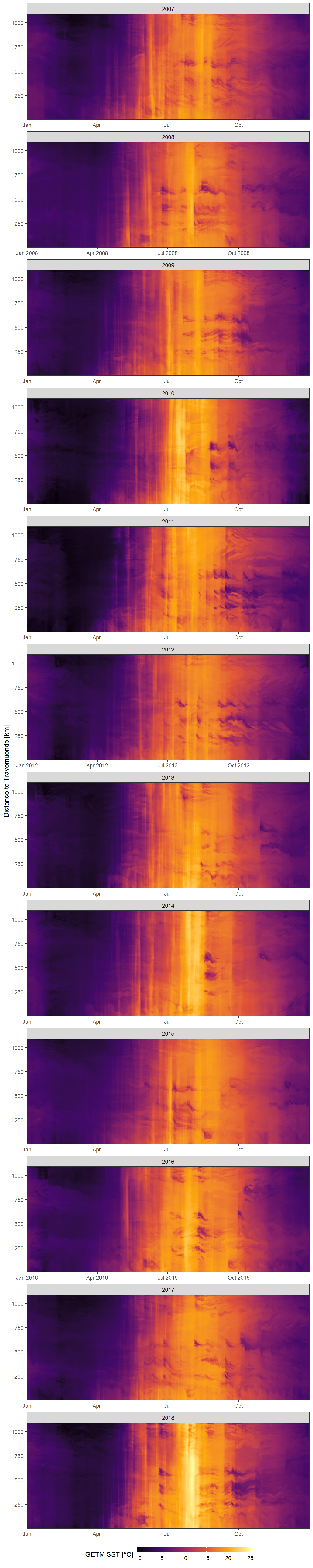

Daily mean GETM SST as a function of time and the ships distance to Travemuende along route E.

3.4.2 Weekly Finnmaid SST

Hovmoeller Plots are generated with ggplot and geom_raster. On the x axis we find the date, the y axis represents the distance to Travemuend in kilometers and the color coding represents weekly mean values of Finnmaid SST.

comparison_gt_fm_sst_hov <-
   vroom::vroom(here::here("data/_merged_data_files/", file = "comparison_gt_fm_sst_hov.csv"))

comparison_gt_fm_sst_hov <- comparison_gt_fm_sst_hov %>% 
  mutate(year = year(week),
         week = as.Date(week))

comparison_gt_fm_sst_hov %>%
  filter(year > 2006, year < 2019) %>% 
    ggplot()+
    geom_raster(aes(week, dist.trav, fill=value_SST_Finn_mean))+
    #scale_fill_scico(palette = "vik", name="mean difference in SST [°C]")+
    scale_fill_viridis_c(name="Finnmaid SST [°C]", na.value = "white", option = "B")+
    scale_x_date(expand = c(0,0))+
    scale_y_continuous(expand = c(0,0))+
    labs(y="Distance to Travemuende [km]")+
    theme_bw()+
    theme(
      axis.title.x = element_blank(),
      legend.position = "bottom",
      legend.key.width = unit(1.3, "cm"),
      legend.key.height = unit(0.3, "cm")
    )+
    facet_wrap(~year, ncol = 1, scales = "free_x")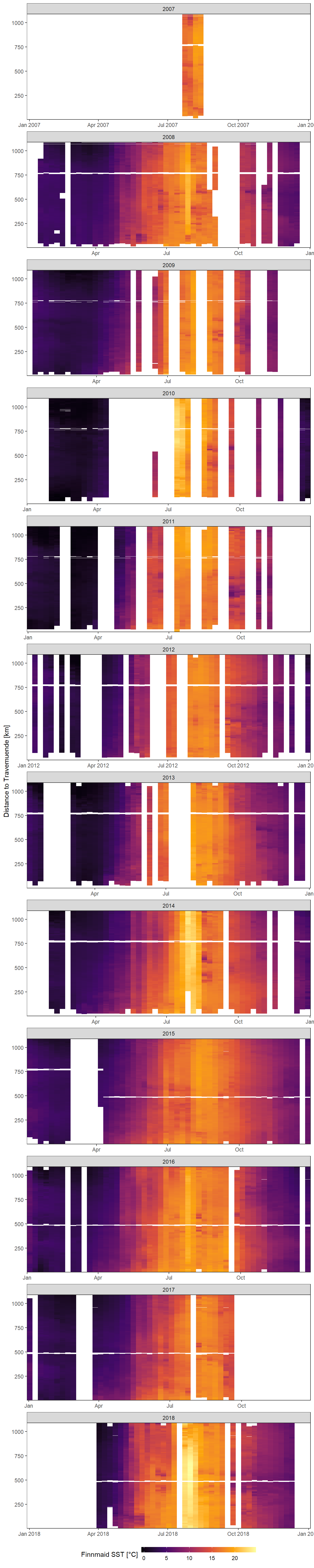

Mean weekly observed (Finnmaid) SST as a function of time and the ships distance to Travemuende along route E.

3.4.3 SST difference

Hovmoeller Plots are generated with ggplot and geom_raster. On the x axis we find the date, the y axis represents the distance to Travemuend in kilometers and the color coding represents the difference between SST GETM and Finnmaid values. In this plot we can see, whether the model produces higher differences in certain areas for example.

comparison_gt_fm_sst_hov %>%
  filter(year > 2006, year < 2019) %>% 
    ggplot()+
    geom_raster(aes(week, dist.trav, fill=difference_mean))+
    #scale_fill_scico(palette = "vik", name="mean difference in SST [°C]")+
    scale_fill_divergent(name="Mean weekly SST difference FM-GETM [°C]", na.value = "white",
                         mid = 'grey')+
    scale_x_date(expand = c(0,0))+
    scale_y_continuous(expand = c(0,0))+
    labs(y="Distance to Travemuende [km]")+
    theme_bw()+
    theme(
      axis.title.x = element_blank(),
      legend.position = "bottom",
      legend.key.width = unit(1.3, "cm"),
      legend.key.height = unit(0.3, "cm")
    )+
    facet_wrap(~year, ncol = 1, scales = "free_x")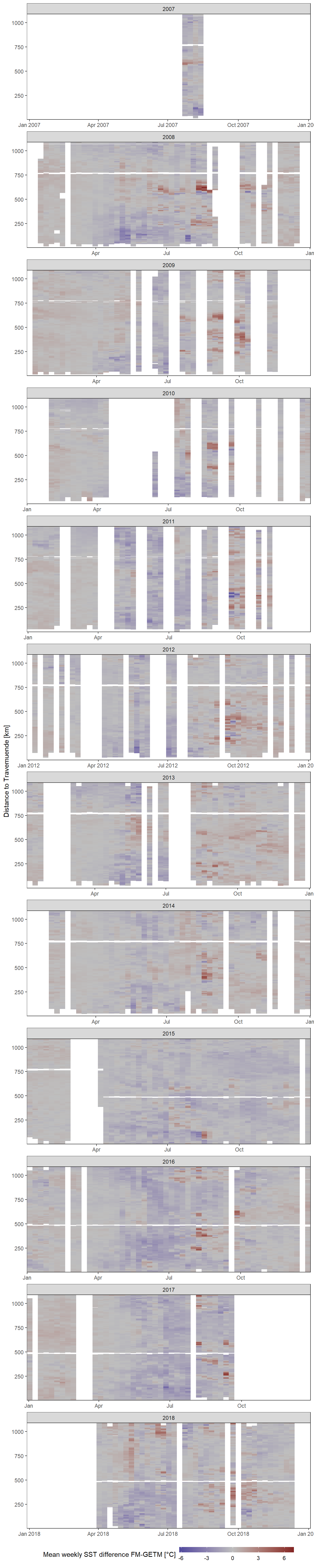

Mean weekly difference between modelled (GETM) and observed (Finnmaid) SST as a function of time and the ships distance to Travemuende along route E.

rm(comparison_gt_fm_sst_hov)

Session information

sessionInfo()

R version 3.6.3 (2020-02-29)
Platform: i386-w64-mingw32/i386 (32-bit)
Running under: Windows 10 x64 (build 18363)

Matrix products: default

locale:
[1] LC_COLLATE=English_Germany.1252  LC_CTYPE=English_Germany.1252   
[3] LC_MONETARY=English_Germany.1252 LC_NUMERIC=C                    
[5] LC_TIME=English_Germany.1252    

attached base packages:
[1] stats     graphics  grDevices utils     datasets  methods   base     

other attached packages:
 [1] metR_0.6.0       here_0.1         xts_0.12-0       zoo_1.8-7       
 [5] dygraphs_1.1.1.6 geosphere_1.5-10 lubridate_1.7.4  vroom_1.2.0     
 [9] ncdf4_1.17       forcats_0.5.0    stringr_1.4.0    dplyr_0.8.5     
[13] purrr_0.3.3      readr_1.3.1      tidyr_1.0.2      tibble_3.0.0    
[17] ggplot2_3.3.0    tidyverse_1.3.0  workflowr_1.6.1 

loaded via a namespace (and not attached):
 [1] Rcpp_1.0.4        whisker_0.4       knitr_1.28        xml2_1.3.0       
 [5] magrittr_1.5      hms_0.5.3         rvest_0.3.5       tidyselect_1.0.0 
 [9] bit_1.1-15.2      viridisLite_0.3.0 colorspace_1.4-1  lattice_0.20-41  
[13] R6_2.4.1          rlang_0.4.5       fansi_0.4.1       parallel_3.6.3   
[17] broom_0.5.5       xfun_0.12         dbplyr_1.4.2      modelr_0.1.6     
[21] withr_2.1.2       git2r_0.26.1      ellipsis_0.3.0    htmltools_0.4.0  
[25] assertthat_0.2.1  bit64_0.9-7       rprojroot_1.3-2   digest_0.6.25    
[29] lifecycle_0.2.0   haven_2.2.0       rmarkdown_2.1     sp_1.4-1         
[33] compiler_3.6.3    cellranger_1.1.0  pillar_1.4.3      scales_1.1.0     
[37] backports_1.1.5   generics_0.0.2    jsonlite_1.6.1    httpuv_1.5.2     
[41] pkgconfig_2.0.3   rstudioapi_0.11   munsell_0.5.0     highr_0.8        
[45] httr_1.4.1        tools_3.6.3       grid_3.6.3        nlme_3.1-145     
[49] data.table_1.12.8 gtable_0.3.0      checkmate_2.0.0   DBI_1.1.0        
[53] cli_2.0.2         readxl_1.3.1      yaml_2.2.1        crayon_1.3.4     
[57] farver_2.0.3      later_1.0.0       promises_1.1.0    htmlwidgets_1.5.1
[61] fs_1.4.0          vctrs_0.2.4       glue_1.3.2        evaluate_0.14    
[65] labeling_0.3      reprex_0.3.0      stringi_1.4.6