Integrated CDR Efficiency Plots
Victoria Froh & Jens Daniel Müller
07 April, 2025
Last updated: 2025-04-07
Checks: 7 0
Knit directory: oae_ccs_roms/
This reproducible R Markdown analysis was created with workflowr (version 1.7.1). The Checks tab describes the reproducibility checks that were applied when the results were created. The Past versions tab lists the development history.
Great! Since the R Markdown file has been committed to the Git repository, you know the exact version of the code that produced these results.
Great job! The global environment was empty. Objects defined in the global environment can affect the analysis in your R Markdown file in unknown ways. For reproduciblity it’s best to always run the code in an empty environment.
The command set.seed(20240919) was run prior to running
the code in the R Markdown file. Setting a seed ensures that any results
that rely on randomness, e.g. subsampling or permutations, are
reproducible.
Great job! Recording the operating system, R version, and package versions is critical for reproducibility.
Nice! There were no cached chunks for this analysis, so you can be confident that you successfully produced the results during this run.
Great job! Using relative paths to the files within your workflowr project makes it easier to run your code on other machines.
Great! You are using Git for version control. Tracking code development and connecting the code version to the results is critical for reproducibility.
The results in this page were generated with repository version 5a5f21a. See the Past versions tab to see a history of the changes made to the R Markdown and HTML files.
Note that you need to be careful to ensure that all relevant files for
the analysis have been committed to Git prior to generating the results
(you can use wflow_publish or
wflow_git_commit). workflowr only checks the R Markdown
file, but you know if there are other scripts or data files that it
depends on. Below is the status of the Git repository when the results
were generated:
Ignored files:
    Ignored:    .Rhistory
    Ignored:    .Rproj.user/

Untracked files:
    Untracked:  code/dist_maps.R
    Untracked:  code/flux_driver_correlations.Rmd
    Untracked:  code/flux_drivers_calcs.R
    Untracked:  code/lineplot_stacks.R
    Untracked:  code/subregions.Rmd
    Untracked:  surface_dataRG2.feather

Unstaged changes:
    Modified:   code/Workflowr_project_managment.R
    Modified:   code/regrid_surface_data.R
    Modified:   code/temperature_indices.Rmd
Note that any generated files, e.g. HTML, png, CSS, etc., are not included in this status report because it is ok for generated content to have uncommitted changes.
These are the previous versions of the repository in which changes were
made to the R Markdown (analysis/cdreff_plots.Rmd) and HTML
(docs/cdreff_plots.html) files. If you’ve configured a
remote Git repository (see ?wflow_git_remote), click on the
hyperlinks in the table below to view the files as they were in that
past version.
| File | Version | Author | Date | Message |
|---|---|---|---|---|
| Rmd | 5a5f21a | vgfroh | 2025-04-07 | Final code push |
| html | 91e2272 | vgfroh | 2025-02-19 | Build site. |
| Rmd | a36bcfe | vgfroh | 2025-02-19 | Mixing depth and air-sea co2 flux anlaysis |
| html | dd18a78 | vgfroh | 2025-02-03 | Build site. |
| Rmd | 639b38d | vgfroh | 2025-02-03 | Column integrated plots and hovmoeller plots completed |
| html | ce19057 | vgfroh | 2025-01-05 | Build site. |
| Rmd | 009b735 | vgfroh | 2025-01-05 | Plotted time series of integrated dTA and CDREff data |
#Introduction
Plotting the results of the full-grid integrated time series of dTA, CDR efficiency, and dDIC for each 3 phases and the mean
#loading packages
library(tidyverse)
library(data.table)
library(arrow)

# Path to intermediate computation outputs
path_outputs <- "/net/sea/work/vifroh/oae_ccs_roms_data/original_grid/"

# Path to save practice plots when working on them
path_plots <- "/net/sea/work/vifroh/test_plots/"

# loading in previous saved integrated CDR data
lanina_cdreff_sum <- read_feather(
  paste0(path_outputs, "lanina_CDReff_integrated.feather"))
neutral_cdreff_sum <- read_feather(
  paste0(path_outputs, "neutral_CDReff_integrated.feather"))
elnino_cdreff_sum <- read_feather(
  paste0(path_outputs, "elnino_CDReff_integrated.feather"))
# create combined table with "phase" column to identify each of the 3
full_cdreff <- rbindlist(
list(lanina = lanina_cdreff_sum, neutral = neutral_cdreff_sum,
elnino = elnino_cdreff_sum),
idcol = "phase")
# add column for months since oae addition begins for x-axis
full_cdreff <- full_cdreff[, month := seq_len(.N), by = phase]
# computing means
full_cdreff[, ":=" (
dTA_mean = mean(dTA_sum, na.rm = TRUE),
dDIC_mean = mean(dDIC_sum, na.rm = TRUE),
CDReff_mean = mean(CDR_eff, na.rm = TRUE)
), by = month]
# save
# write_feather(full_cdreff, paste0(path_outputs,
# "full_CDReff_integrated.feather"))Integrated Line Plots of 3 Phases
# plotting dTA
ggplot(full_cdreff, aes(x = month, y = dTA_sum/1e10, color = phase)) +
  scale_x_continuous(breaks = seq(6, 72, by = 6), limits = c(0,72),
                     expand = c(0,0)) +
  scale_y_continuous(limits = c(0, 19), expand = c(0,0)) +
  geom_vline(xintercept = 12, linetype = "dashed", color = "grey75", linewidth = 0.6) +
  geom_hline(yintercept = 16.7, linetype = "dashed", color = "black", linewidth = 0.6) +
  geom_line(linewidth = 1) +
  scale_color_discrete(labels = c("elnino" = "El Niño", "lanina" = "La Niña", "neutral" = "Neutral")
  ) +
  labs(x = "Months Since OAE Start",
       y = "Integrated TA' [10\u00B9\u2070 mol]" #, title = "Total Added Alkalinity"
       ) +
  theme_bw() +
  theme(panel.grid = element_blank(), legend.position = c(0.875, 0.2),
        legend.text = element_text(size = 15),
        legend.box.background = element_rect(color = "grey80", size = 0.5),
        axis.text = element_text(size = 15, color = "black"),
        axis.title = element_text(size = 16),
        plot.title = element_blank(), legend.title = element_blank(),
        axis.ticks = element_line(color = "black", size = 0.5),
        axis.ticks.length = unit(0.3, "cm"),
        panel.border = element_rect(color = "black", size = 0.5),
        plot.margin = margin(15, 15, 15, 15)) +
  coord_cartesian(clip = 'off', expand = FALSE)
Warning: The `size` argument of `element_line()` is deprecated as of ggplot2 3.4.0.
ℹ Please use the `linewidth` argument instead.
This warning is displayed once every 8 hours.
Call `lifecycle::last_lifecycle_warnings()` to see where this warning was
generated.Warning: The `size` argument of `element_rect()` is deprecated as of ggplot2 3.4.0.
ℹ Please use the `linewidth` argument instead.
This warning is displayed once every 8 hours.
Call `lifecycle::last_lifecycle_warnings()` to see where this warning was
generated.Warning: A numeric `legend.position` argument in `theme()` was deprecated in ggplot2
3.5.0.
ℹ Please use the `legend.position.inside` argument of `theme()` instead.
This warning is displayed once every 8 hours.
Call `lifecycle::last_lifecycle_warnings()` to see where this warning was
generated.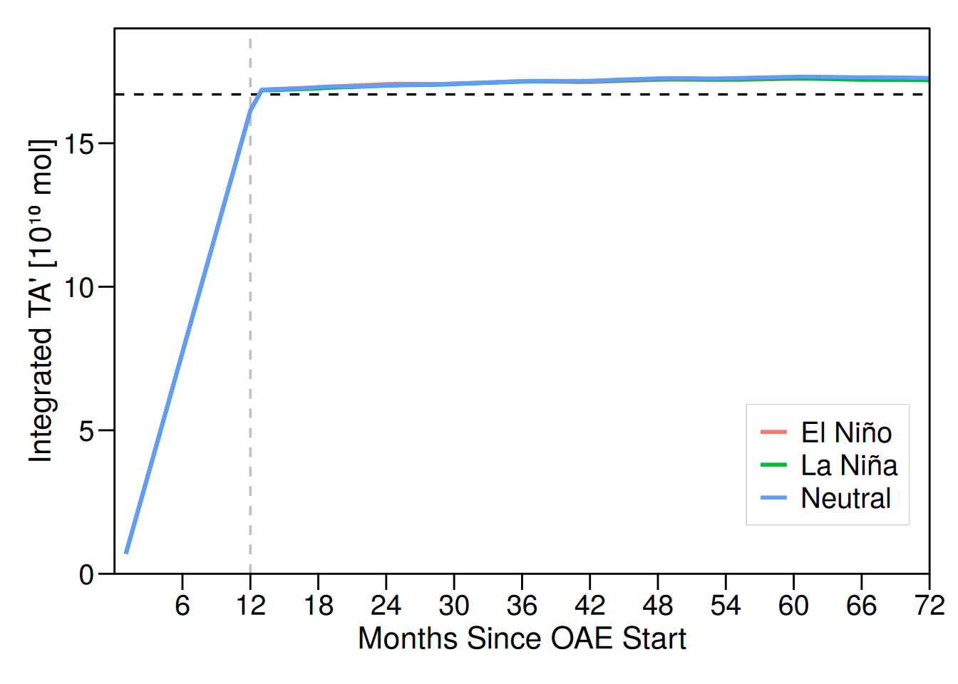
# ggsave(paste0(path_plots, "total_dTA_cum.png"), plot = last_plot(),
#               width = 6, height = 4, dpi = 300)

# plotting CDReff
ggplot(full_cdreff, aes(x = month, y = CDR_eff, color = phase)) +
  geom_vline(xintercept = 12, linetype = "dashed", color = "grey75", linewidth = 0.6) +
  geom_line(linewidth = 1) +
  scale_x_continuous(breaks = seq(6, 72, by = 6), limits = c(0, 72),
                     expand = c(0, 0)) +
  scale_y_continuous(limits = c(0, 1), expand = c(0, 0)) +
  scale_color_discrete(labels = c("elnino" = "El Niño", "lanina" = "La Niña", "neutral" = "Neutral")
  ) +
  labs(x = "Months Since OAE Start",
       y = "Integrated \u03B7" #, title = "Integrated CDR Efficiency"
       ) +
  theme_bw() +
  theme(panel.grid = element_blank(), legend.position = c(0.87, 0.2),
        legend.text = element_text(size = 15),
        legend.box.background = element_rect(color = "grey80", size = 0.5),
        axis.text = element_text(size = 15, color = "black"),
        axis.title = element_text(size = 16),
        plot.title = element_blank(), legend.title = element_blank(),
        axis.ticks = element_line(color = "black", size = 0.5),
        axis.ticks.length = unit(0.3, "cm"),
        panel.border = element_rect(color = "black", size = 0.5),
        plot.margin = margin(15, 15, 15, 15)) +
  coord_cartesian(clip = 'off', expand = FALSE)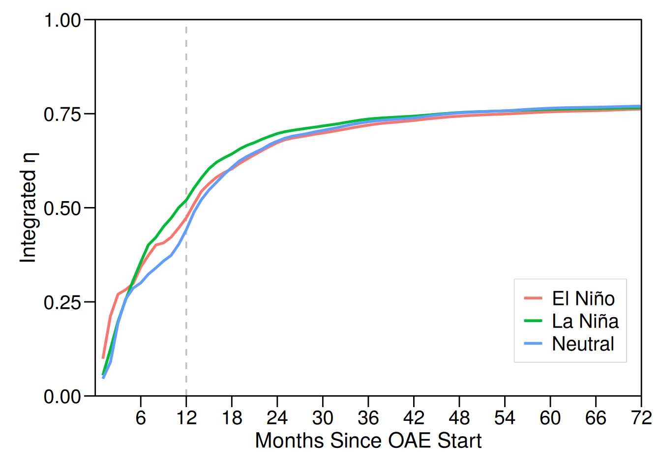
# ggsave(paste0(path_plots, "CDReff_int.png"), plot = last_plot(),
#               width = 6, height = 4, dpi = 300)

# plotting dDIC
ggplot(full_cdreff, aes(x = month, y = dDIC_sum/1e10, color = phase)) +
  scale_x_continuous(breaks = seq(6, 72, by = 6), limits = c(0,72),
                     expand = c(0,0)) +
  scale_y_continuous(limits = c(0, 19), expand = c(0,0)) +
  geom_vline(xintercept = 12, linetype = "dashed", color = "grey75", linewidth = 0.6) +
  geom_hline(yintercept = 13.36, linetype = "dashed", color = "black", linewidth = 0.6) +
  geom_line(linewidth = 1) +
  scale_color_discrete(labels = c("elnino" = "El Niño", "lanina" = "La Niña", "neutral" = "Neutral")
  ) +
  labs(x = "Months Since OAE Start",
       y = "Integrated DIC' [10\u00B9\u2070 mol]" #, title = "Total Change in Dissolved Inorganic Carbon"
       ) +
  theme_bw() +
  theme(panel.grid = element_blank(), legend.position = c(0.875, 0.2),
        legend.text = element_text(size = 15),
        legend.box.background = element_rect(color = "grey80", size = 0.5),
        axis.text = element_text(size = 15, color = "black"),
        axis.title = element_text(size = 16),
        plot.title = element_blank(), legend.title = element_blank(),
        axis.ticks = element_line(color = "black", size = 0.5),
        axis.ticks.length = unit(0.3, "cm"),
        panel.border = element_rect(color = "black", size = 0.5),
        plot.margin = margin(15, 15, 15, 15)) +
  coord_cartesian(clip = 'off', expand = FALSE)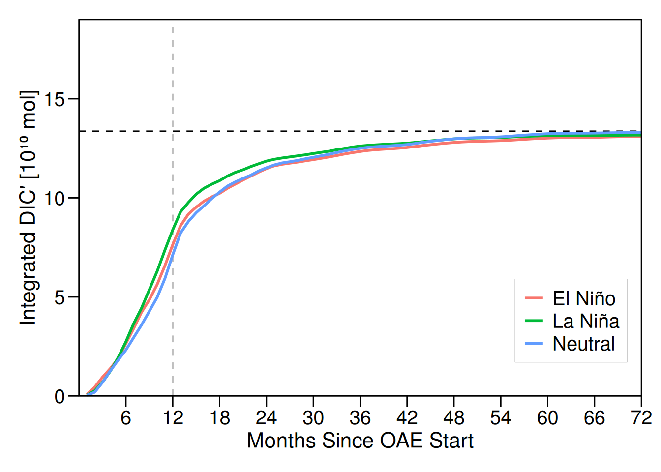
| Version | Author | Date |
|---|---|---|
| 91e2272 | vgfroh | 2025-02-19 |
# ggsave(paste0(path_plots, "total_dDIC_cum.png"), plot = last_plot(),
#               width = 6, height = 4, dpi = 300)
Integrated Line Plots of Means
# to add a shaded ribbon showing the range:
full_cdreff <- full_cdreff[, ':='(
  min_TA = min(dTA_sum), max_TA = max(dTA_sum),
  min_DIC = min(dDIC_sum), max_DIC = max(dDIC_sum),
  min_eff = min(CDR_eff), max_eff = max(CDR_eff)
), by = month]


# plotting dTA
ggplot(full_cdreff, aes(x = month, y = dTA_mean/1e10)) +
  scale_x_continuous(breaks = seq(6, 72, by = 6), limits = c(0,72),
                     expand = c(0,0)) +
  scale_y_continuous(limits = c(0, 19), expand = c(0,0)) +
  geom_vline(xintercept = 12, linetype = "dashed", color = "grey75", linewidth = 0.6) +
  geom_hline(yintercept = 16.7, linetype = "dashed", color = "black", linewidth = 0.6) +
  geom_ribbon(aes(ymin = min_TA/1e10, ymax = max_TA/1e10), fill = "#A6CEE3", alpha = 0.45) +
  geom_line(linewidth = 1) +
  labs(x = "Months Since OAE Start",
       y = " Mean Integrated TA' [10\u00B9\u2070 mol]" #,  title = "Mean Total Added Alkalinity"
       ) +
  theme_bw() +
  theme(panel.grid = element_blank(), #legend.position = c(0.9, 0.2),
        # legend.text = element_text(size = 12),
        # legend.box.background = element_rect(color = "grey80", size = 0.5),
        axis.text = element_text(size = 13, color = "black"),
        axis.title = element_text(size = 15),
        plot.title = element_blank(), legend.title = element_blank(),
        axis.ticks = element_line(color = "black", size = 0.5),
        axis.ticks.length = unit(0.3, "cm"),
        panel.border = element_rect(color = "black", size = 0.5),
        plot.margin = margin(15, 15, 15, 15)) +
  coord_cartesian(clip = 'off', expand = FALSE)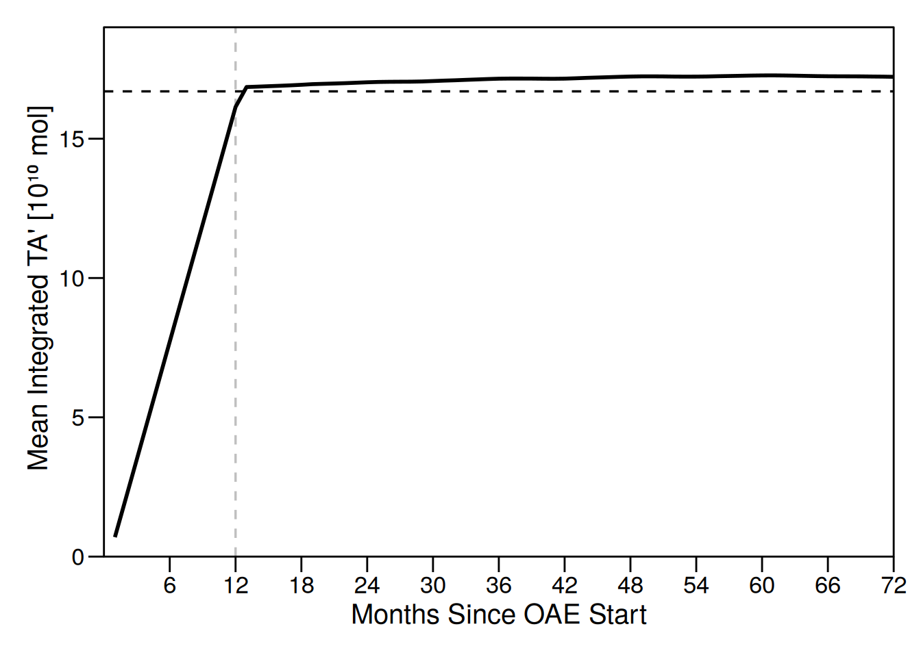
# ggsave(paste0(path_plots, "total_dTA_cum_mean.png"), plot = last_plot(),
#               width = 8, height = 4, dpi = 300)

# plotting CDReff
ggplot(full_cdreff, aes(x = month, y = CDReff_mean)) +
  geom_vline(xintercept = 12, linetype = "dashed", color = "grey75", linewidth = 0.6) +
  geom_ribbon(aes(ymin = min_eff, ymax = max_eff), fill = "#A6CEE3", alpha = 0.45) +
  geom_line(linewidth = 1) +
  scale_x_continuous(breaks = seq(6, 72, by = 6), limits = c(0, 72),
                     expand = c(0, 0)) +
  scale_y_continuous(limits = c(0, 1), expand = c(0, 0)) +
  labs(x = "Months Since OAE Start",
       y = "Mean Integrated \u03B7" #, title = "Mean Integrated CDR Efficiency"
       ) +
  theme_bw() +
  theme(panel.grid = element_blank(), #legend.position = c(0.9, 0.2),
        # legend.text = element_text(size = 12),
        # legend.box.background = element_rect(color = "grey80", size = 0.5),
        axis.text = element_text(size = 13, color = "black"),
        axis.title = element_text(size = 15),
        plot.title = element_blank(), legend.title = element_blank(),
        axis.ticks = element_line(color = "black", size = 0.5),
        axis.ticks.length = unit(0.3, "cm"),
        panel.border = element_rect(color = "black", size = 0.5),
        plot.margin = margin(15, 15, 15, 15)) +
  coord_cartesian(clip = 'off', expand = FALSE)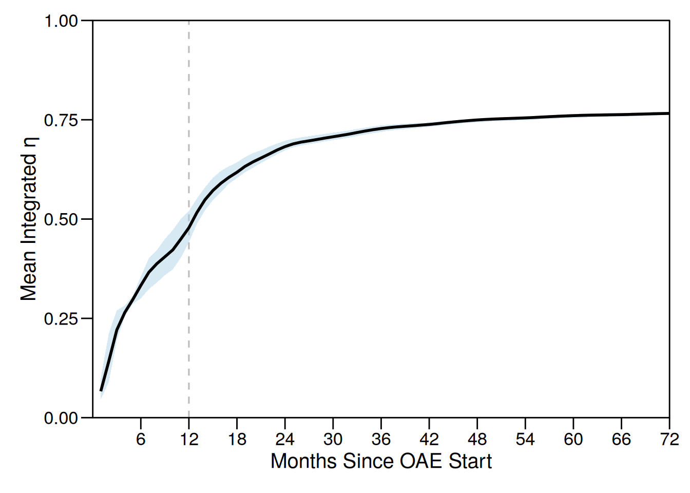
# ggsave(paste0(path_plots, "CDReff_int_mean.png"), plot = last_plot(),
#               width = 8, height = 4, dpi = 300)

# plotting dDIC
ggplot(full_cdreff, aes(x = month, y = dDIC_mean/1e10)) +
  scale_x_continuous(breaks = seq(6, 72, by = 6), limits = c(0,72),
                     expand = c(0,0)) +
  scale_y_continuous(limits = c(0, 19), expand = c(0,0)) +
  geom_vline(xintercept = 12, linetype = "dashed", color = "grey75", linewidth = 0.6) +
  geom_hline(yintercept = 13.36, linetype = "dashed", color = "black", linewidth = 0.6) +
  geom_ribbon(aes(ymin = min_DIC/1e10, ymax = max_DIC/1e10), fill = "#A6CEE3", alpha = 0.45) +
  geom_line(linewidth = 1) +
  labs(x = "Months Since OAE Start",
       y = "Mean Integrated DIC' [10\u00B9\u2070 mol]" #, title = "Mean Total New Dissolved Inorganic Carbon"
       ) +
  theme_bw() +
  theme(panel.grid = element_blank(), #legend.position = c(0.9, 0.2),
        # legend.text = element_text(size = 12),
        # legend.box.background = element_rect(color = "grey80", size = 0.5),
        axis.text = element_text(size = 13, color = "black"),
        axis.title = element_text(size = 15),
        plot.title = element_blank(), legend.title = element_blank(),
        axis.ticks = element_line(color = "black", size = 0.5),
        axis.ticks.length = unit(0.3, "cm"),
        panel.border = element_rect(color = "black", size = 0.5),
        plot.margin = margin(15, 15, 15, 15)) +
  coord_cartesian(clip = 'off', expand = FALSE)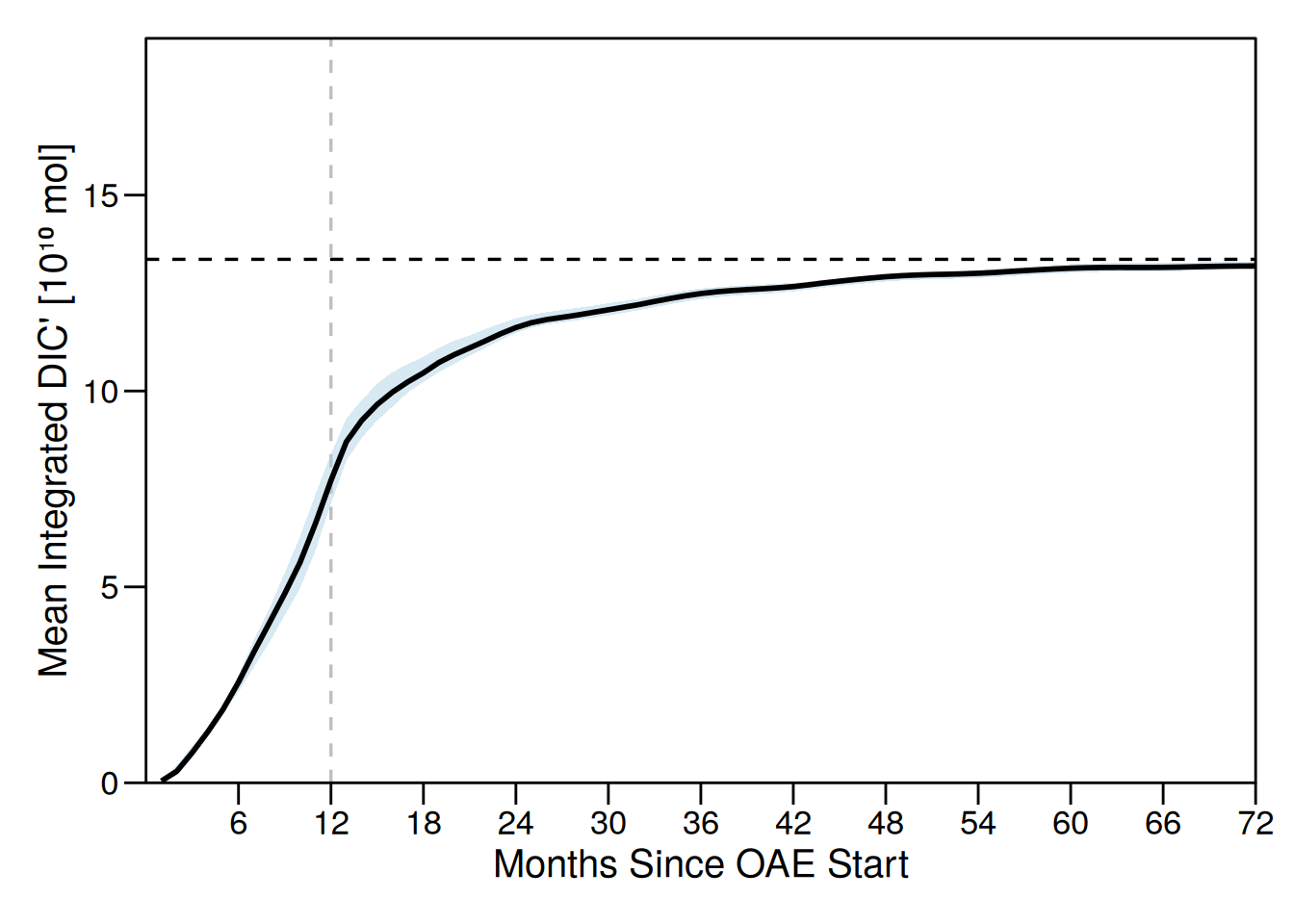
# ggsave(paste0(path_plots, "total_dDIC_cum_mean.png"), plot = last_plot(),
#               width = 8, height = 4, dpi = 300)
Difference from Mean Plots
# plotting dTA
ggplot(full_cdreff, aes(x = month, y = (dTA_sum - dTA_mean)/1e10, color = phase)) +
  scale_x_continuous(breaks = seq(6, 72, by = 6), limits = c(0,72),
                     expand = c(0,0)) +
  scale_y_continuous(limits = c(-1, 1), expand = c(0,0)) +
  geom_vline(xintercept = 12, linetype = "dashed", color = "grey75", linewidth = 0.6) +
  #geom_hline(yintercept = 16.7, linetype = "dashed", color = "black", linewidth = 0.6) +
  geom_line(linewidth = 1) +
  scale_color_discrete(labels = c("elnino" = "El Niño", "lanina" = "La Niña", "neutral" = "Neutral")
  ) +
  labs(x = "Months Since OAE Start",
       y = "Integrated \u0394TA' [10\u00B9\u2070 mol]" #, title = "Total Added Alkalinity"
       ) +
  theme_bw() +
  theme(panel.grid = element_blank(), legend.position = c(0.875, 0.2),
        legend.text = element_text(size = 15),
        legend.box.background = element_rect(color = "grey80", size = 0.5),
        axis.text = element_text(size = 15, color = "black"),
        axis.title = element_text(size = 16),
        plot.title = element_blank(), legend.title = element_blank(),
        axis.ticks = element_line(color = "black", size = 0.5),
        axis.ticks.length = unit(0.3, "cm"),
        panel.border = element_rect(color = "black", size = 0.5),
        plot.margin = margin(15, 15, 15, 15)) +
  coord_cartesian(clip = 'off', expand = FALSE)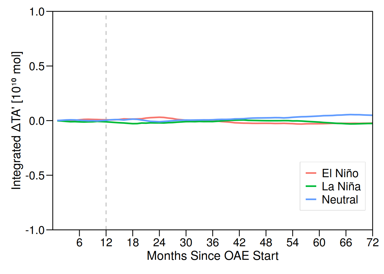
# ggsave(paste0(path_plots, "total_dTA_cum_dfm.png"), plot = last_plot(),
#               width = 6, height = 4, dpi = 300)

# plotting CDReff
ggplot(full_cdreff, aes(x = month, y = CDR_eff - CDReff_mean, color = phase)) +
  geom_vline(xintercept = 12, linetype = "dashed", color = "grey75", linewidth = 0.6) +
  geom_line(linewidth = 1) +
  scale_x_continuous(breaks = seq(6, 72, by = 6), limits = c(0, 72),
                     expand = c(0, 0)) +
  scale_y_continuous(limits = c(-.1, .1), expand = c(0, 0)) +
  scale_color_discrete(labels = c("elnino" = "El Niño", "lanina" = "La Niña", "neutral" = "Neutral")
  ) +
  labs(x = "Months Since OAE Start",
       y = "Integrated \u0394\u03B7" #, title = "Integrated CDR Efficiency"
       ) +
  theme_bw() +
  theme(panel.grid = element_blank(), legend.position = c(0.87, 0.2),
        legend.text = element_text(size = 15),
        legend.box.background = element_rect(color = "grey80", size = 0.5),
        axis.text = element_text(size = 15, color = "black"),
        axis.title = element_text(size = 16),
        plot.title = element_blank(), legend.title = element_blank(),
        axis.ticks = element_line(color = "black", size = 0.5),
        axis.ticks.length = unit(0.3, "cm"),
        panel.border = element_rect(color = "black", size = 0.5),
        plot.margin = margin(15, 15, 15, 15)) +
  coord_cartesian(clip = 'off', expand = FALSE)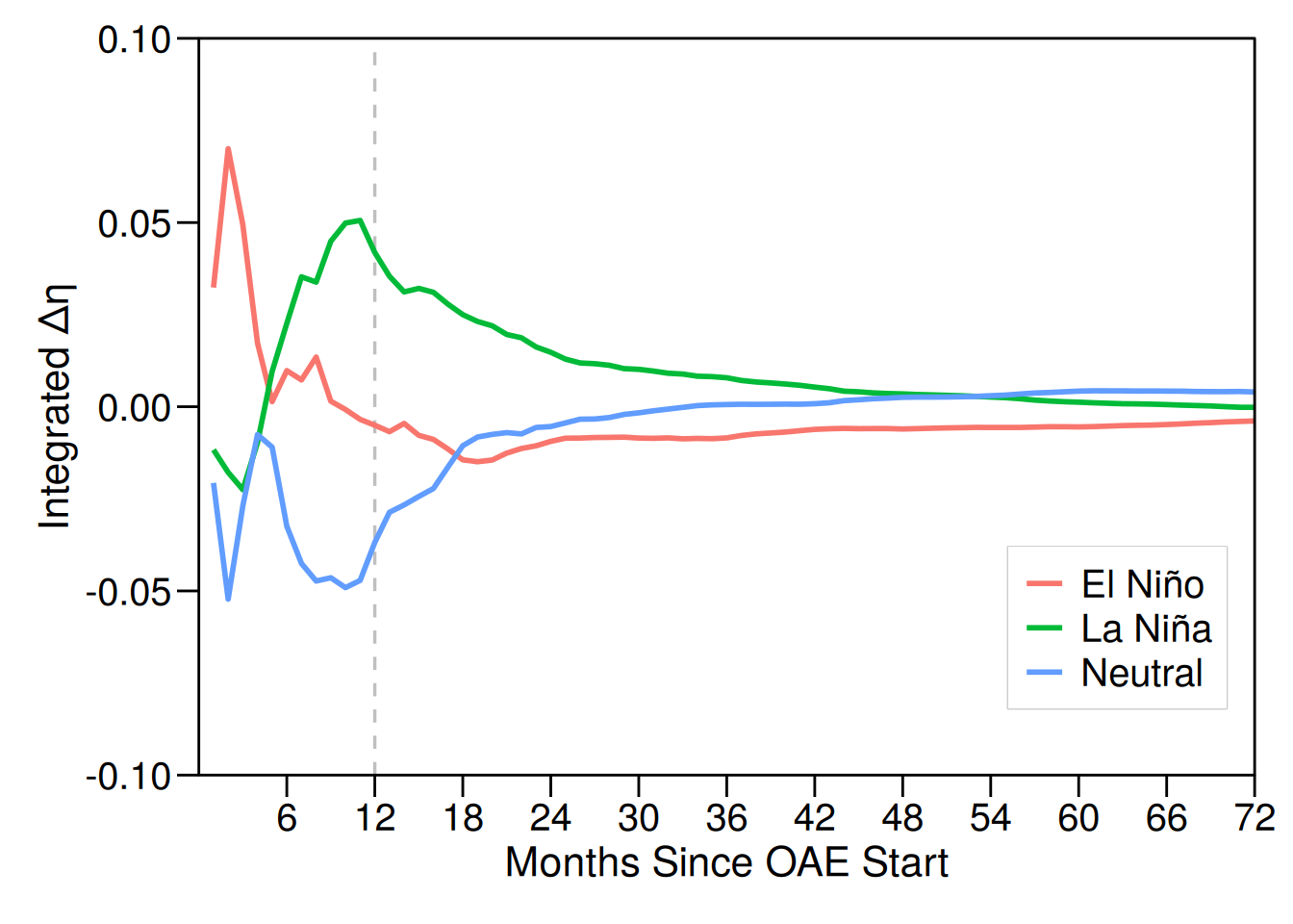
# ggsave(paste0(path_plots, "CDReff_int_dfm.png"), plot = last_plot(),
#               width = 6, height = 4, dpi = 300)

# plotting dDIC
ggplot(full_cdreff, aes(x = month, y = (dDIC_sum - dDIC_mean)/1e10, color = phase)) +
  scale_x_continuous(breaks = seq(6, 72, by = 6), limits = c(0,72),
                     expand = c(0,0)) +
  scale_y_continuous(limits = c(-1, 1), expand = c(0,0)) +
  geom_vline(xintercept = 12, linetype = "dashed", color = "grey75", linewidth = 0.6) +
  #geom_hline(yintercept = 13.36, linetype = "dashed", color = "black", linewidth = 0.6) +
  geom_line(linewidth = 1) +
  scale_color_discrete(labels = c("elnino" = "El Niño", "lanina" = "La Niña", "neutral" = "Neutral")
  ) +
  labs(x = "Months Since OAE Start",
       y = "Integrated \u0394DIC' [10\u00B9\u2070 mol]" #, title = "Total Change in Dissolved Inorganic Carbon"
       ) +
  theme_bw() +
  theme(panel.grid = element_blank(), legend.position = c(0.875, 0.2),
        legend.text = element_text(size = 15),
        legend.box.background = element_rect(color = "grey80", size = 0.5),
        axis.text = element_text(size = 15, color = "black"),
        axis.title = element_text(size = 16),
        plot.title = element_blank(), legend.title = element_blank(),
        axis.ticks = element_line(color = "black", size = 0.5),
        axis.ticks.length = unit(0.3, "cm"),
        panel.border = element_rect(color = "black", size = 0.5),
        plot.margin = margin(15, 15, 15, 15)) +
  coord_cartesian(clip = 'off', expand = FALSE)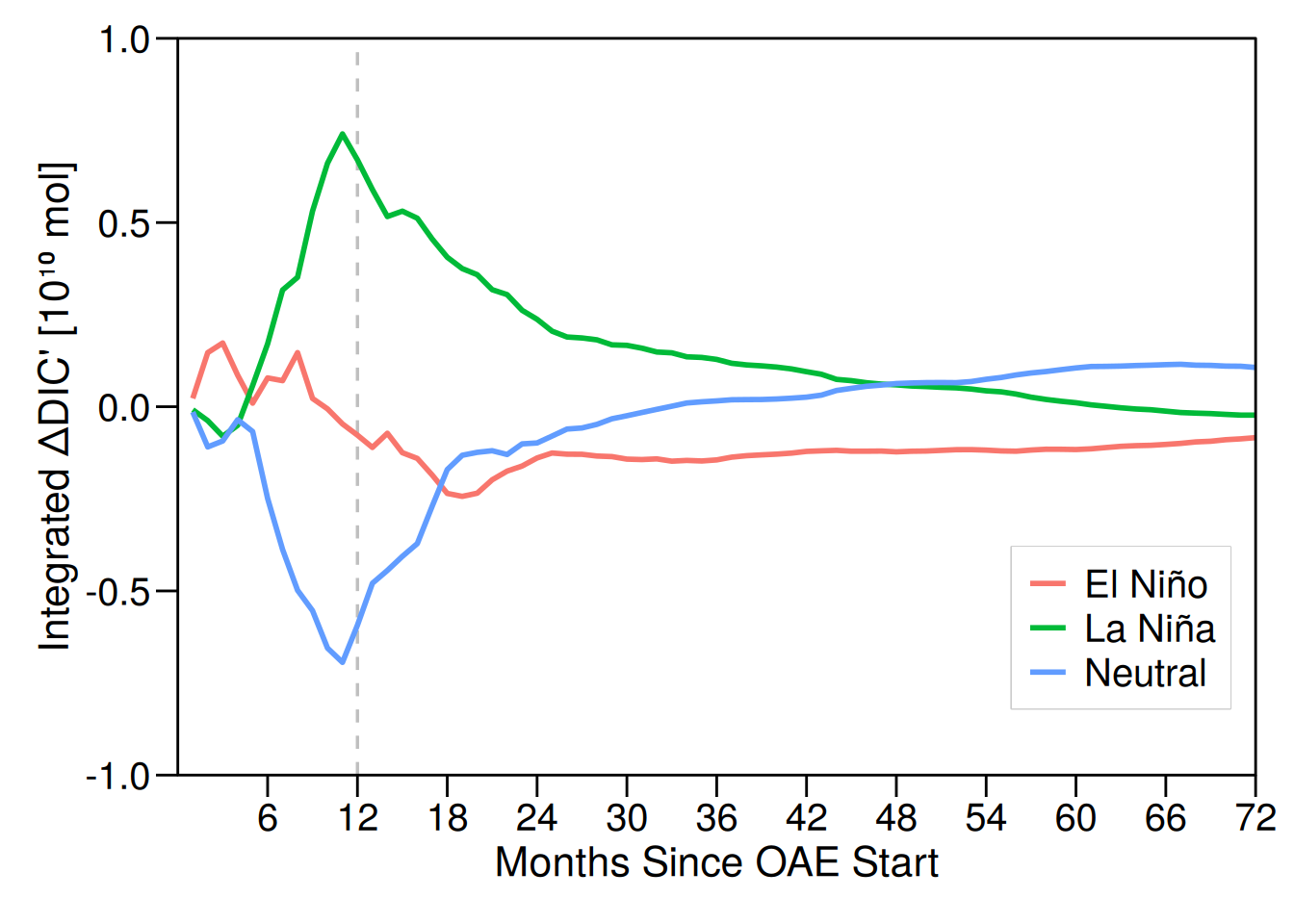
# ggsave(paste0(path_plots, "total_dDIC_cum_dfm.png"), plot = last_plot(),
#               width = 6, height = 4, dpi = 300)

rm(list = ls())
gc()
used (Mb) gc trigger (Mb) max used (Mb)
Ncells 1688229 90.2 3260507 174.2 3260507 174.2
Vcells 2981135 22.8 8388608 64.0 6327066 48.3
sessionInfo()R version 4.4.2 (2024-10-31)
Platform: x86_64-pc-linux-gnu
Running under: openSUSE Leap 15.6
Matrix products: default
BLAS/LAPACK: /usr/local/OpenBLAS-0.3.28/lib/libopenblas_haswellp-r0.3.28.so; LAPACK version 3.12.0
locale:
[1] LC_CTYPE=en_US.UTF-8 LC_NUMERIC=C
[3] LC_TIME=en_US.UTF-8 LC_COLLATE=en_US.UTF-8
[5] LC_MONETARY=en_US.UTF-8 LC_MESSAGES=en_US.UTF-8
[7] LC_PAPER=en_US.UTF-8 LC_NAME=C
[9] LC_ADDRESS=C LC_TELEPHONE=C
[11] LC_MEASUREMENT=en_US.UTF-8 LC_IDENTIFICATION=C
time zone: Europe/Zurich
tzcode source: system (glibc)
attached base packages:
[1] stats graphics grDevices utils datasets methods base
other attached packages:
[1] arrow_18.1.0.1 data.table_1.16.2 lubridate_1.9.3 forcats_1.0.0
[5] stringr_1.5.1 dplyr_1.1.4 purrr_1.0.2 readr_2.1.5
[9] tidyr_1.3.1 tibble_3.2.1 ggplot2_3.5.1 tidyverse_2.0.0
[13] workflowr_1.7.1
loaded via a namespace (and not attached):
[1] sass_0.4.9 utf8_1.2.4 generics_0.1.3 stringi_1.8.4
[5] hms_1.1.3 digest_0.6.37 magrittr_2.0.3 timechange_0.3.0
[9] evaluate_1.0.1 grid_4.4.2 fastmap_1.2.0 rprojroot_2.0.4
[13] jsonlite_1.8.9 processx_3.8.4 whisker_0.4.1 ps_1.8.1
[17] promises_1.3.2 httr_1.4.7 fansi_1.0.6 scales_1.3.0
[21] jquerylib_0.1.4 cli_3.6.3 crayon_1.5.3 rlang_1.1.4
[25] bit64_4.5.2 munsell_0.5.1 withr_3.0.2 cachem_1.1.0
[29] yaml_2.3.10 tools_4.4.2 tzdb_0.4.0 colorspace_2.1-1
[33] httpuv_1.6.15 assertthat_0.2.1 vctrs_0.6.5 R6_2.5.1
[37] lifecycle_1.0.4 git2r_0.35.0 bit_4.5.0 fs_1.6.5
[41] pkgconfig_2.0.3 callr_3.7.6 pillar_1.9.0 bslib_0.8.0
[45] later_1.4.1 gtable_0.3.6 glue_1.8.0 Rcpp_1.0.13-1
[49] xfun_0.49 tidyselect_1.2.1 rstudioapi_0.17.1 knitr_1.49
[53] farver_2.1.2 htmltools_0.5.8.1 labeling_0.4.3 rmarkdown_2.29
[57] compiler_4.4.2 getPass_0.2-4