NCP best guess
Jens Daniel Müller
02 July, 2021
Last updated: 2021-07-02
Checks: 7 0
Knit directory: BloomSail/
This reproducible R Markdown analysis was created with workflowr (version 1.6.2). The Checks tab describes the reproducibility checks that were applied when the results were created. The Past versions tab lists the development history.
Great! Since the R Markdown file has been committed to the Git repository, you know the exact version of the code that produced these results.
Great job! The global environment was empty. Objects defined in the global environment can affect the analysis in your R Markdown file in unknown ways. For reproduciblity it’s best to always run the code in an empty environment.
The command set.seed(20191021) was run prior to running the code in the R Markdown file. Setting a seed ensures that any results that rely on randomness, e.g. subsampling or permutations, are reproducible.
Great job! Recording the operating system, R version, and package versions is critical for reproducibility.
Nice! There were no cached chunks for this analysis, so you can be confident that you successfully produced the results during this run.
Great job! Using relative paths to the files within your workflowr project makes it easier to run your code on other machines.
Great! You are using Git for version control. Tracking code development and connecting the code version to the results is critical for reproducibility.
The results in this page were generated with repository version 0fb46b7. See the Past versions tab to see a history of the changes made to the R Markdown and HTML files.
Note that you need to be careful to ensure that all relevant files for the analysis have been committed to Git prior to generating the results (you can use wflow_publish or wflow_git_commit). workflowr only checks the R Markdown file, but you know if there are other scripts or data files that it depends on. Below is the status of the Git repository when the results were generated:
Ignored files:
    Ignored:    .Rhistory
    Ignored:    .Rproj.user/
    Ignored:    data/

Untracked files:
    Untracked:  data_bg-2021-40_resubmission.zip
    Untracked:  output/Plots/Figures_publication/.tmp.drivedownload/
    Untracked:  output/Plots/Figures_publication/Article_wo_P07-P10/
Note that any generated files, e.g. HTML, png, CSS, etc., are not included in this status report because it is ok for generated content to have uncommitted changes.
These are the previous versions of the repository in which changes were made to the R Markdown (analysis/NCP_best_guess.Rmd) and HTML (docs/NCP_best_guess.html) files. If you’ve configured a remote Git repository (see ?wflow_git_remote), click on the hyperlinks in the table below to view the files as they were in that past version.
| File | Version | Author | Date | Message |
|---|---|---|---|---|
| Rmd | 0fb46b7 | jens-daniel-mueller | 2021-07-02 | rerun with NE stations |
| html | 484d5e1 | jens-daniel-mueller | 2021-07-02 | Build site. |
| Rmd | 386d322 | jens-daniel-mueller | 2021-07-02 | test without NE stations |
| html | ae96bc0 | jens-daniel-mueller | 2021-06-30 | Build site. |
| Rmd | aa9fd37 | jens-daniel-mueller | 2021-06-30 | adapted plot design |
| html | c8a1425 | jens-daniel-mueller | 2021-05-18 | Build site. |
| html | 00a2574 | jens-daniel-mueller | 2021-05-10 | Build site. |
| html | b19a1fb | jens-daniel-mueller | 2021-05-10 | Build site. |
| Rmd | c438b10 | jens-daniel-mueller | 2021-05-10 | removed grid lines |
| html | b5d6ad3 | jens-daniel-mueller | 2021-05-10 | Build site. |
| Rmd | d3c1469 | jens-daniel-mueller | 2021-05-10 | removed grid lines |
| Rmd | 4f593fe | jens-daniel-mueller | 2021-05-10 | removed grid lines |
| html | 61e452c | jens-daniel-mueller | 2021-04-16 | Build site. |
| html | 2f64f92 | jens-daniel-mueller | 2021-03-30 | Build site. |
| Rmd | 23acb8c | jens-daniel-mueller | 2021-03-30 | revised figure according to RC1 |
| html | 4a1065b | jens-daniel-mueller | 2021-03-30 | Build site. |
| Rmd | a520c10 | jens-daniel-mueller | 2021-03-30 | revised figure according to RC1 |
| html | 82145cc | jens-daniel-mueller | 2021-02-20 | Build site. |
| Rmd | ac99c61 | jens-daniel-mueller | 2021-02-20 | cleaning |
| html | 5f4fb9a | jens-daniel-mueller | 2021-02-20 | Build site. |
| Rmd | 031f46a | jens-daniel-mueller | 2021-02-20 | rerun with early exclusion of negative pCO2 |
| html | 516b294 | jens-daniel-mueller | 2021-02-18 | Build site. |
| Rmd | 233bbc1 | jens-daniel-mueller | 2021-02-18 | rerun all with empty folders |
| html | 3d08cda | jens-daniel-mueller | 2021-02-18 | Build site. |
| Rmd | c909ee0 | jens-daniel-mueller | 2021-02-18 | cleaning |
| html | a9d3656 | jens-daniel-mueller | 2021-02-18 | Build site. |
| Rmd | 391e9bd | jens-daniel-mueller | 2021-02-18 | cleaning |
| html | a2e2485 | jens-daniel-mueller | 2021-02-18 | Build site. |
| Rmd | 4959ab4 | jens-daniel-mueller | 2021-02-18 | cleaning |
| html | 195aab4 | jens-daniel-mueller | 2021-02-18 | Build site. |
| Rmd | 4d3eab9 | jens-daniel-mueller | 2021-02-18 | cleaning |
| html | 41bc9c8 | jens-daniel-mueller | 2021-02-16 | Build site. |
| Rmd | b41ec42 | jens-daniel-mueller | 2021-02-16 | added scalebars |
| html | fb3c39e | jens-daniel-mueller | 2021-02-16 | Build site. |
| Rmd | 710be31 | jens-daniel-mueller | 2021-02-16 | cleaning |
| html | 5f838ef | jens-daniel-mueller | 2021-02-16 | Build site. |
| Rmd | ec6ed6b | jens-daniel-mueller | 2021-02-16 | created all profiles pdfs |
| html | 4ab2a50 | jens-daniel-mueller | 2021-02-16 | Build site. |
| Rmd | 23e959a | jens-daniel-mueller | 2021-02-16 | added plot for coastal stations |
| html | 5d19b26 | jens-daniel-mueller | 2021-02-16 | Build site. |
| Rmd | 5cd670b | jens-daniel-mueller | 2021-02-16 | cleaning |
| html | 189f202 | jens-daniel-mueller | 2021-02-16 | Build site. |
| Rmd | 06d5293 | jens-daniel-mueller | 2021-02-16 | cleaning |
| html | cfa3fbf | jens-daniel-mueller | 2021-02-16 | Build site. |
| Rmd | d064708 | jens-daniel-mueller | 2021-02-16 | renamed CT_star |
| html | f8d471f | jens-daniel-mueller | 2021-02-16 | Build site. |
| Rmd | 4ce82b8 | jens-daniel-mueller | 2021-02-16 | added scalebar |
| html | 0af0021 | jens-daniel-mueller | 2021-02-15 | Build site. |
| Rmd | 4878a06 | jens-daniel-mueller | 2021-02-15 | cleaning |
| html | 70a8950 | jens-daniel-mueller | 2021-02-11 | Build site. |
| Rmd | 4bdeb1f | jens-daniel-mueller | 2021-02-11 | rerun all with empty folders |
library(tidyverse)
library(patchwork)
library(seacarb)
library(marelac)
library(metR)
library(scico)
library(lubridate)
library(zoo)
library(tibbletime)
library(sp)
library(kableExtra)
library(LakeMetabolizer)
library(rgdal)
library(ggnewscale)
library(ggsn)
1 Scope of this script
- Analyse field data recorded on board SV Tina V
- Derive a best guess estimate for net community production (NCP)
2 Sensor data
2.1 Data preparation
Profile data are prepared by:
- Ignoring those made on June 16 (pCO2 sensor not in operation)
- Removing HydroC Flush and Zeroing periods
- Selecting only continuous downcast periods
- Gridding profiles to 1m depth intervals
- Removing grids with pCO2 < 0 µatm (presumably RT correction artifact after zeroing)
- Discarding profiles with 20 or more observation missing within upper 25m
- Assigning mean date_time_ID value to all profiles belonging to one cruise
- Discarding “coastal” station P01, P13, P14
- Restricting profiles to upper 25m
Please note that:
- The label ID represents the start date of the cruise (“YYMMDD”), not the exact mean sampling date
tm <-
  read_csv(
    here::here(
      "data/intermediate/_merged_data_files/response_time",
      "tm_RT_all.csv"
    ),
    col_types = cols(
      ID = col_character(),
      pCO2_analog = col_double(),
      pCO2_corr = col_double(),
      Zero = col_character(),
      Flush = col_character(),
      mixing = col_character(),
      Zero_counter = col_integer(),
      deployment = col_integer(),
      lon = col_double(),
      lat = col_double(),
      pCO2 = col_double()
    )
  )


# Filter relevant rows and columns
tm_profiles <- tm %>%
  filter(type == "P",
         Flush == "0",
         Zero == "0",
         !ID %in% parameters$dates_out,
         !(station %in% c("PX1", "PX2"))
         # by uncommenting the line below, you can run the analysis
         # without the NE stations which were affected by lateral water mass exchange
         # ,!(station %in% c("P07", "P08", "P09", "P10"))
         ) %>%
  select(date_time,
         ID,
         station,
         lat,
         lon,
         dep,
         sal,
         tem,
         pCO2_corr,
         pCO2,
         duration)

#calculate mean location of stations
stations <- tm_profiles %>%
  group_by(station) %>%
  summarise(lat = mean(lat),
            lon = mean(lon)) %>%
  ungroup() %>%
  mutate(station = str_sub(station, 2, 3))


# Assign meta information
tm_profiles <- tm_profiles %>%
  group_by(ID, station) %>%
  mutate(duration = as.numeric(date_time - min(date_time))) %>%
  arrange(date_time) %>%
  ungroup()

meta <- read_csv(here::here("data/input/TinaV/Sensor",
                            "Sensor_meta.csv"),
                 col_types = cols(ID = col_character()))

meta <- meta %>%
    filter(!ID %in% parameters$dates_out)

tm_profiles <- full_join(tm_profiles, meta)
rm(meta)


# creating descriptive variables
tm_profiles <- tm_profiles %>%
  mutate(phase = "standby",
         phase = if_else(duration >= start & duration < down & !is.na(down) & !is.na(start),
                         "down", phase),
         phase = if_else(duration >= down  & duration < lift & !is.na(lift) & !is.na(down ),
                         "low",  phase),
         phase = if_else(duration >= lift  & duration < up   & !is.na(up  ) & !is.na(lift  ),
                         "mid",  phase),
         phase = if_else(duration >= up    & duration < end  & !is.na(end ) & !is.na(up   ),
                         "up",   phase))

tm_profiles <- tm_profiles %>%
  select(-c(start, down, lift, up, end, comment, p_type, duration))


# select downcast profiles only
tm_profiles <- tm_profiles %>%
  filter(phase %in% parameters$phases_in)

# grid observation to 1m depth intervals
tm_profiles <- tm_profiles %>%
  mutate(dep_grid = as.numeric(as.character(cut(
    dep, seq(0, 40, 1), seq(0.5, 39.5, 1)
  )))) %>%
  group_by(ID, station, dep_grid, phase) %>%
  summarise_all("mean", na.rm = TRUE) %>%
  ungroup() %>%
  select(-dep, dep = dep_grid)

# subset complete profiles of stations not included in analysis
profiles_stations_out <- tm_profiles %>%
  filter(station %in% c("P14", "P13", "P01"))

profiles_stations_out_in <- profiles_stations_out %>%
  filter(dep < parameters$max_dep_gap,
         phase == "down") %>%
  group_by(ID, station) %>%
  summarise(nr_na = parameters$max_dep_gap/parameters$dep_grid - n()) %>%
  mutate(select = if_else(nr_na < parameters$max_gap,
                          "in", "out")) %>%
  select(-nr_na) %>%
  ungroup()

tm_profiles_stations_out <- full_join(profiles_stations_out_in, profiles_stations_out)
rm(profiles_stations_out, profiles_stations_out_in)


# subset complete profiles of stations included in analysis
tm_profiles <- tm_profiles %>%
  filter(!(station %in% c("P14", "P13", "P01")))

profiles_in <- tm_profiles %>%
  filter(dep < parameters$max_dep_gap,
         phase == "down") %>%
  group_by(ID, station) %>%
  summarise(nr_na = parameters$max_dep_gap/parameters$dep_grid - n()) %>%
  mutate(select = if_else(nr_na < parameters$max_gap,
                          "in", "out")) %>%
  select(-nr_na) %>%
  ungroup()

tm_profiles <- full_join(tm_profiles, profiles_in)

tm_profiles <- tm_profiles %>%
  mutate(select = if_else(is.na(select) | select == "out",
                                "out",
                                "in"))
rm(profiles_in)
2.2 pCO2 profile overview
tm_profiles %>%
  arrange(date_time) %>%
  ggplot(aes(pCO2, dep, col = select, linetype = phase)) +
  geom_hline(yintercept = 25) +
  geom_path() +
  scale_y_reverse() +
  scale_x_continuous(breaks = c(0, 600), labels = c(0, 600)) +
  scale_color_brewer(palette = "Set1", direction = -1) +
  coord_cartesian(xlim = c(0, 600)) +
  facet_grid(ID ~ station)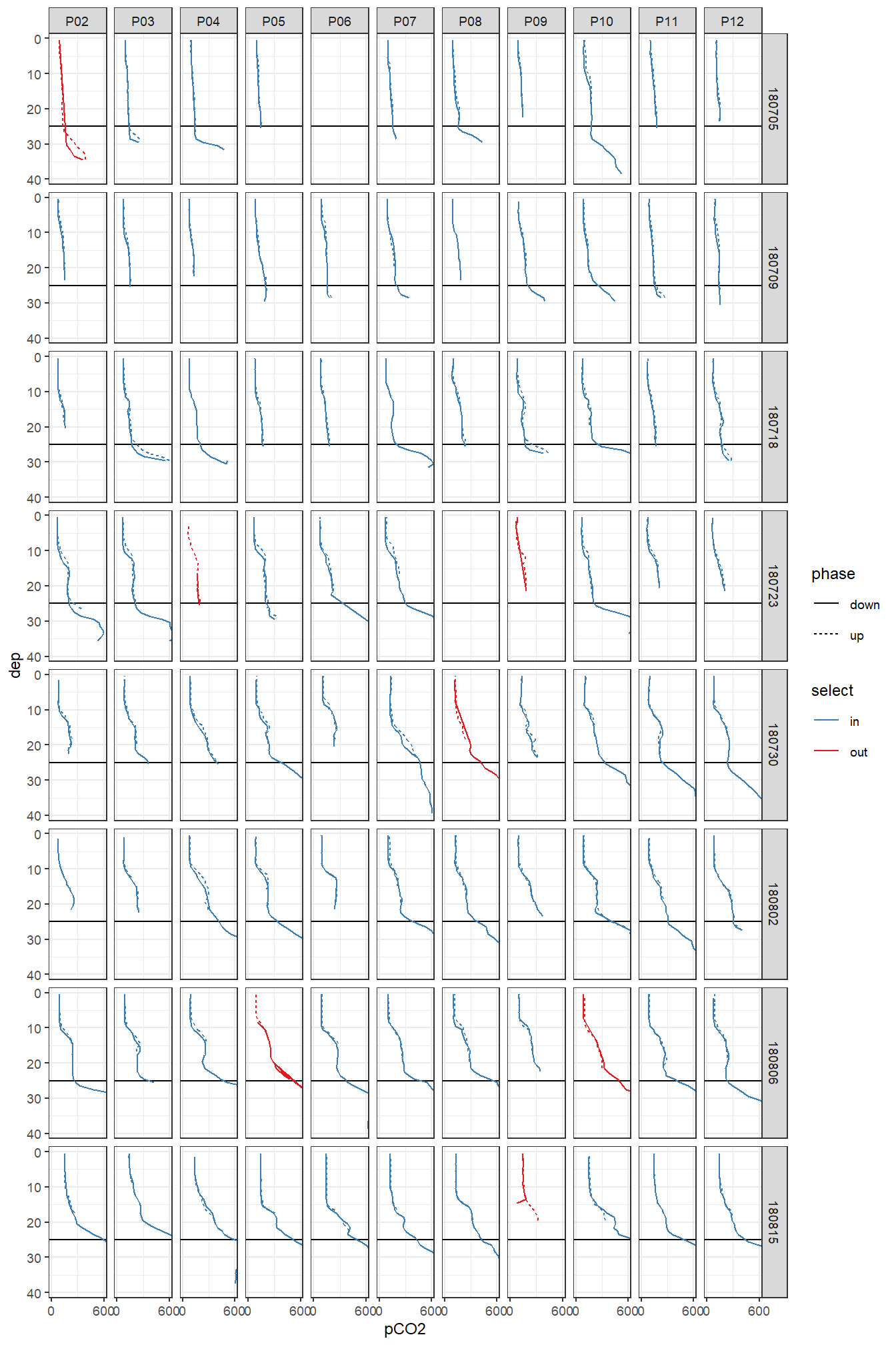
Overview pCO2 profiles at stations (P02-P12) and cruise dates (ID). y-axis restricted to displayed range.
tm_profiles %>%
  group_by(select) %>%
  summarise(nr = n_distinct(ID, station)) %>%
  ungroup()
# A tibble: 2 x 2
select nr
<chr> <int>
1 in 79
2 out 72.3 Subset
tm_profiles <- tm_profiles %>%
  filter(select == "in",
         phase == "down") %>%
  select(-c(select, phase)) %>%
  filter(dep < parameters$max_dep)
2.4 Calculate mean cruise dates
# assign mean date_time stamp
cruise_dates <- tm_profiles %>%
  group_by(ID) %>%
  summarise(date_time_ID = mean(date_time),
            date_ID = format(as.Date(date_time_ID), "%b %d")) %>%
  ungroup()

# join profiles and mean date
tm_profiles <- inner_join(cruise_dates, tm_profiles)

cruise_dates %>%
    write_csv(here::here("data/intermediate/_summarized_data_files",
                       "cruise_date.csv"))
2.5 Station map
2.5.1 Load SOOP Finnmaid data
# read file
fm <-
  read_csv(here::here("data/intermediate/_summarized_data_files",
                      "fm.csv"))

# filter data inside map
fm <- fm %>%
  filter(
    lat <= parameters$map_lat_hi,
    lat >= parameters$map_lat_lo,
    lon >= parameters$map_lon_lo
  )

# tag data inside study area to be analyzed
fm <- fm %>%
  mutate(
    Area = point.in.polygon(
      point.x = lon,
      point.y = lat,
      pol.x = parameters$fm_box_lon,
      pol.y = parameters$fm_box_lat
    ),
    Area = as.character(Area),
    Area = if_else(Area == "1", "utilized", "sampled")
  )

# write tagged data to be analyzed in NCP reconstruction
fm %>%
  filter(Area == "utilized") %>%
  select(-Area) %>%
  write_csv(here::here(
    "data/intermediate/_summarized_data_files",
    "fm_bloomsail.csv"
  ))
2.5.2 Load MODIS satellite image
# handling of the satellite image was inspired by this website:
# https://shekeine.github.io/visualization/2014/09/27/sfcc_rgb_in_R
# https://www.neonscience.org/resources/learning-hub/tutorials/dc-multiband-rasters-r

# read raster file manually downloaded from:
# https://worldview.earthdata.nasa.gov/

EGS  <-
  raster::stack(here::here("data/input/Maps",
                   "MODIS_2018_07_26_EGS.tiff"))

# convert to tibble
EGS <- raster::as.data.frame(EGS, xy = T)
EGS <- as_tibble(EGS)

# rename coordinates and subset region
EGS <- EGS %>%
  rename(lat = y,
         lon = x) %>%
  filter(lat >= 56.4, lat <= 58.3)

# stretch histograms of each band and convert to RGB color
EGS <- EGS %>%
  mutate(
    MODIS_2018_07_26_EGS.1_s = MODIS_2018_07_26_EGS.1 * 2.5,
    MODIS_2018_07_26_EGS.2_s = MODIS_2018_07_26_EGS.2 * 2.5,
    MODIS_2018_07_26_EGS.3_s = MODIS_2018_07_26_EGS.3 * 2.5
  ) %>%
  mutate(
    MODIS_2018_07_26_EGS.1_s =
      if_else(MODIS_2018_07_26_EGS.1_s > 255,
              255,
              MODIS_2018_07_26_EGS.1_s),
    MODIS_2018_07_26_EGS.2_s =
      if_else(MODIS_2018_07_26_EGS.2_s > 255,
              255,
              MODIS_2018_07_26_EGS.2_s),
    MODIS_2018_07_26_EGS.3_s =
      if_else(MODIS_2018_07_26_EGS.3_s > 255,
              255,
              MODIS_2018_07_26_EGS.3_s)) %>%
      mutate(
        RGB = rgb(
          MODIS_2018_07_26_EGS.1_s,
          MODIS_2018_07_26_EGS.2_s,
          MODIS_2018_07_26_EGS.3_s,
          maxColorValue = 255
        )
      )

# select relevant columns
EGS <- EGS %>%
  select(-c(
    MODIS_2018_07_26_EGS.1,
    MODIS_2018_07_26_EGS.2,
    MODIS_2018_07_26_EGS.3
  )) %>%
  select(-c(
    MODIS_2018_07_26_EGS.1_s,
    MODIS_2018_07_26_EGS.2_s,
    MODIS_2018_07_26_EGS.3_s
  ))

# plot map
EGS <- EGS %>%
  rename(long = lon)

p_MODIS <-
  ggplot(data = EGS,
         aes(long, lat, fill = RGB)) +
  coord_quickmap(expand = 0) +
  geom_raster() +
  scale_fill_identity() +
  annotate(
    "rect",
    ymax = parameters$map_lat_hi,
    ymin = parameters$map_lat_lo,
    xmax = parameters$map_lon_hi,
    xmin = parameters$map_lon_lo,
    fill = NA,
    color = "orangered",
    size = 1.5
  ) +
  scale_x_continuous(breaks = seq(10, 30, 1)) +
  labs(x = "Longitude (°E)", y = "Latitude (°N)") +
  scalebar(
    EGS,
    transform = TRUE,
    model = "WGS84",
    dist_unit = "nm",
    dist = 25,
    location = "bottomleft",
    anchor = c(x = 17, y = 56.6),
    st.dist = 0.05,
    st.size = geom_text_size,
    st.color = "white",
    box.color = "white",
    border.size = 0.3
  )
2.5.3 Load bathymetric map
# read file
map <-
  read_csv(here::here("data/input/Maps", "Bathymetry_Gotland_east_small.csv"))

# filter region for plot
map <- map %>%
  filter(
    lat < parameters$map_lat_hi,
    lat > parameters$map_lat_lo,
    lon < parameters$map_lon_hi,
    lon > parameters$map_lon_lo
  )

# adjust resolution
map_low_res <- map %>%
  mutate(
    lat = cut(
      lat,
      breaks = seq(57, 58, 0.01),
      labels = seq(57.005, 57.995, 0.01)
    ),
    lon = cut(
      lon,
      breaks = seq(18, 22, 0.01),
      labels = seq(18.005, 21.995, 0.01)
    )
  ) %>%
  group_by(lat, lon) %>%
  summarise_all(mean, na.rm = TRUE) %>%
  ungroup() %>%
  mutate(lat = as.numeric(as.character(lat)),
         lon = as.numeric(as.character(lon))) %>%
  rename(long = lon)

# downsize track data for plot
tm_track <- tm %>%
  arrange(date_time) %>%
  slice(which(row_number() %% 10 == 1))


# plot map
p_map <-
  ggplot() +
  geom_contour_fill(
    data = map_low_res,
    aes(x = long, y = lat, z = -elev),
    na.fill = TRUE,
    breaks = seq(0, 300, 30)
  ) +
  geom_raster(data = map %>% filter(is.na(elev)),
              aes(lon, lat),
              fill = "darkgrey") +
  geom_path(data = tm_track, aes(lon, lat, group = ID, col = "Data\nused")) +
  scale_color_manual(values = c("orangered"),
                     name = "") +
  new_scale_color() +
  geom_path(data = tm_track, aes(lon, lat, group = ID, col = "sampled")) +
  geom_path(data = fm, aes(lon, lat, group = ID, col = Area)) +
  geom_label(
    data = stations %>% filter(!(station %in% c("14", "13", "01"))),
    aes(lon, lat, label = station, col = "utilized"),
    size = geom_text_size
  ) +
  geom_label(
    data = stations %>% filter(station %in% c("14", "13", "01")),
    aes(lon, lat, label = station, col = "sampled_station"),
    size = geom_text_size
  ) +
  geom_point(aes(parameters$herrvik_lon, parameters$herrvik_lat)) +
  geom_text(
    aes(parameters$herrvik_lon, parameters$herrvik_lat, label = "Herrvik"),
    nudge_x = -0.05,
    nudge_y = -0.01,
    size = geom_text_size
  ) +
  geom_point(aes(parameters$ostergarn_lon, parameters$ostergarn_lat)) +
  geom_text(
    aes(parameters$ostergarn_lon, parameters$ostergarn_lat,
        label = "Östergarnsholm\nFlux tower"),
    nudge_x = -0.07,
    nudge_y = 0.03,
    size = geom_text_size
  ) +
  geom_text(aes(19.26, 57.57, label = "SOOP Finnmaid"),
            col = "white",
            size = geom_text_size) +
  geom_text(aes(19.54, 57.29, label = "SV Tina V"),
            col = "white",
            size = geom_text_size) +
  coord_quickmap(
    expand = 0,
    ylim = c(parameters$map_lat_lo + 0.01, parameters$map_lat_hi - 0.01)
  ) +
  scale_x_continuous(breaks = seq(10, 30, 0.1)) +
  labs(x = "Longitude (°E)", y = "Latitude (°N)") +
  scale_fill_gradient(
    low = "lightsteelblue1",
    high = "dodgerblue4",
    name = "Depth (m)\n",
    breaks = seq(30, 150, 30),
    limits = c(0, 180),
    guide = "colorstrip"
  ) +
  guides(
    fill = guide_colorsteps(
      barheight = unit(35, "mm"),
      barwidth = unit(5, "mm"),
      show.limits = TRUE,
      frame.colour = "black",
      ticks = TRUE,
      ticks.colour = "black"
    )
  ) +
  scale_color_manual(values = c("white", "darkgrey", "orangered"),
                     guide = FALSE) +
  scalebar(
    map_low_res,
    transform = TRUE,
    model = "WGS84",
    dist_unit = "nm",
    dist = 2.5,
    location = "bottomleft",
    anchor = c(x = 18.65, y = 57.3),
    st.dist = 0.05,
    st.size = geom_text_size,
    border.size = 0.3
  )

p_MODIS + p_map +
  plot_layout(ncol = 1) +
  plot_annotation(tag_levels = 'a')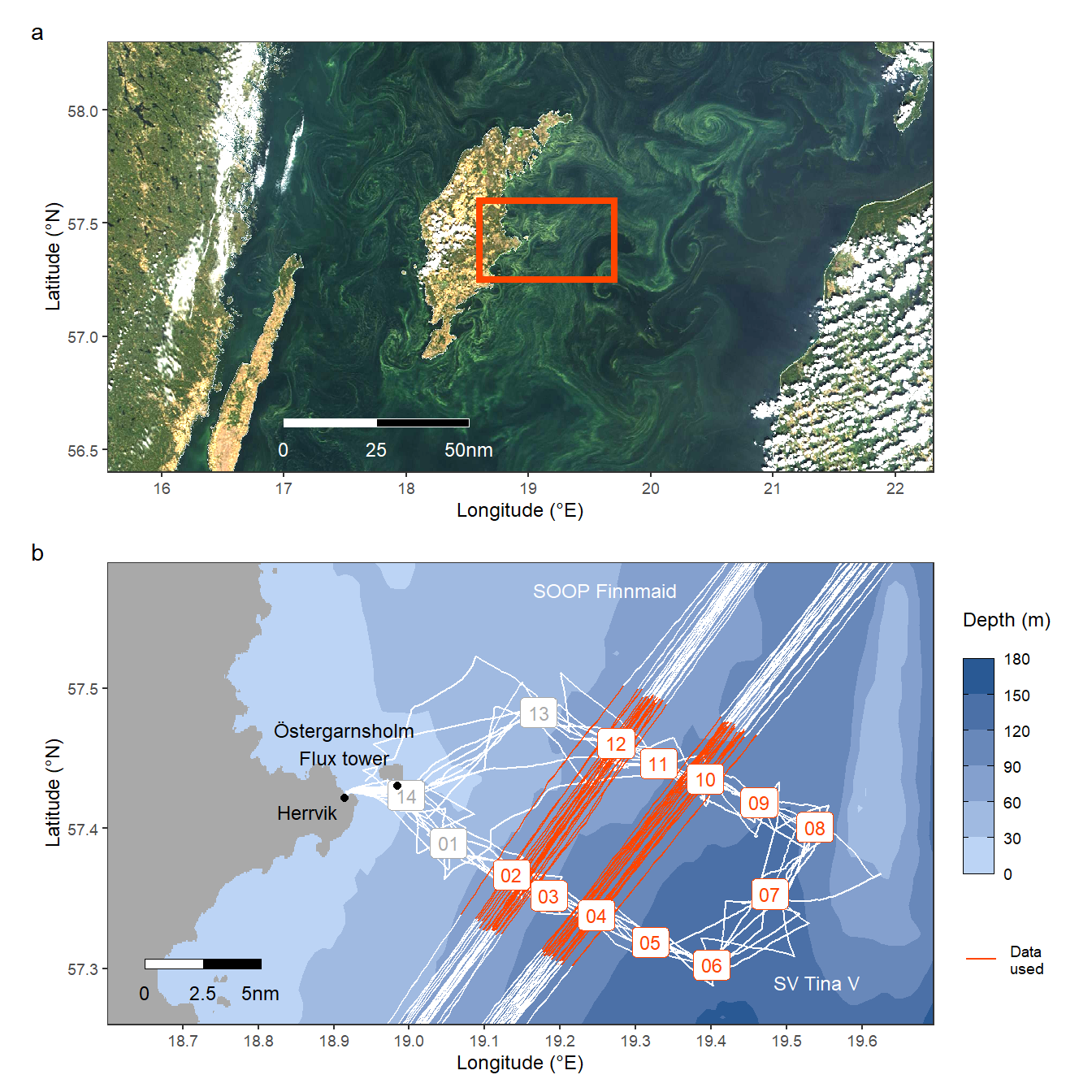
Location of stations sampled between the east coast of Gotland and Gotland deep.
ggsave(
  here::here("output/Plots/Figures_publication/article",
             "Fig_1.pdf"),
  width = 175,
  height = 200,
  dpi = 300,
  units = "mm"
)

ggsave(
  here::here("output/Plots/Figures_publication/article",
             "Fig_1.png"),
  width = 160,
  height = 170,
  dpi = 300,
  units = "mm"
)

rm(map, map_low_res, p_map, p_MODIS,
   fm, tm_track, tm, EGS)
2.6 Data coverage
# calculate mean samppling dates per station
cover <- tm_profiles %>%
  group_by(ID, station) %>%
  summarise(date = mean(date_time),
            date_time_ID = mean(date_time_ID)) %>%
  ungroup() %>%
  mutate(station = str_sub(station, 2, 3))

# create coverage plot
cover %>%
  ggplot(aes(date, station, fill = ID)) +
  geom_vline(aes(xintercept = date_time_ID, col = ID)) +
  geom_point(shape = 21) +
  scale_fill_viridis_d(labels = cruise_dates$date_ID,
                       name = "Mean\ncruise date") +
  scale_color_viridis_d(labels = cruise_dates$date_ID,
                        name = "Mean\ncruise date") +
  scale_x_datetime(date_breaks = "week",
                   date_labels = "%b %d") +
  labs(y = "Station") +
  theme(axis.title.x = element_blank(),
        panel.grid.major.x = element_blank(),
        panel.grid.minor.x = element_blank())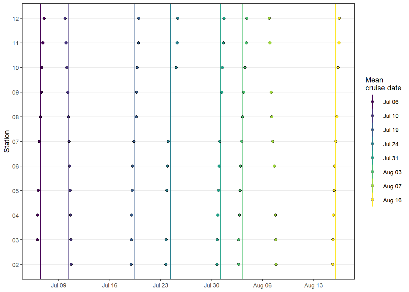
Spatio-temporal data coverage, indicated as station visits over time.
ggsave(
  here::here(
    "output/Plots/Figures_publication/article",
    "Fig_2.pdf"
  ),
  width = 100,
  height = 65,
  dpi = 300,
  units = "mm"
)

ggsave(
  here::here(
    "output/Plots/Figures_publication/article",
    "Fig_2.png"
  ),
  width = 100,
  height = 65,
  dpi = 300,
  units = "mm"
)

rm(cover)
3 Bottle CT and AT
At stations P07 and P10 discrete samples for lab measurments of CT and AT were collected. Please note that - in contrast to the pCO2 profiles - samples were taken on June 16, but removed here for harmonization of results.
# read files
tb <-
  read_csv(
    here::here("data/intermediate/_summarized_data_files", "tb.csv"),
    col_types = cols(ID = col_character())
  )

# select stations, harmonize depth range and date ID
tb <- tb %>%
  filter(station %in% c("P07", "P10"),
         dep <= parameters$max_dep) %>%
  mutate(ID = if_else(ID == "180722", "180723", ID))

# join with mean cruise dates
tb <- inner_join(tb, cruise_dates)
3.1 Mean AT
In order to derive CT from measured pCO2 profiles, the alkalinity mean + sd in the upper 25m and both stations was calculated as:
# AT mean calculation
AT_mean <- tb %>%
  filter(dep <= parameters$max_dep) %>%
  summarise(AT = mean(AT, na.rm = TRUE)) %>%
  pull()

AT_mean
[1] 1719.706# AT SD calculation
AT_sd <- tb %>%
filter(dep <= parameters$max_dep) %>%
summarise(AT = sd(AT, na.rm = TRUE)) %>%
pull()
AT_sd[1] 26.957713.2 Mean Salinity
Likewise, the mean salinity amounts to:
# Sal mean calculation
sal_mean <- tb %>%
  filter(dep <= parameters$max_dep) %>%
  summarise(sal = mean(sal, na.rm = TRUE)) %>%
  pull()

sal_mean
[1] 6.908356tb_fix <- bind_cols(start = min(tm_profiles$date_time),
end = max(tm_profiles$date_time),
AT = AT_mean,
AT_sd = AT_sd,
sal = sal_mean)
tb_fix %>%
write_csv(here::here("data/intermediate/_summarized_data_files", "tb_fix.csv"))3.3 CT* calculation
The alkalinity-normalized CT, CT*, was calculated for discrete samples.
# calculate CT*, referred to as CT_star in the code
tb <- tb %>%
  mutate(CT_star = CT/AT * AT_mean)
3.4 Vertical profiles
3.4.1 Stations
tb_long <- tb %>%
  pivot_longer(c(sal:AT, CT_star), names_to = "var", values_to = "value")

tb_long %>%
  ggplot(aes(value, dep)) +
  geom_path(aes(col = ID)) +
  geom_point(aes(fill = ID), shape = 21) +
  scale_y_reverse() +
  scale_fill_viridis_d(labels = cruise_dates$date_ID) +
  scale_color_viridis_d(labels = cruise_dates$date_ID) +
  facet_grid(station ~ var, scales = "free_x") +
  theme(legend.position = "bottom",
        legend.title = element_blank())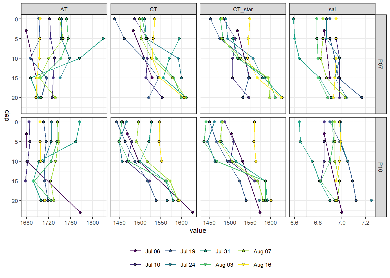
Discrete sample profiles for individual stations
3.4.2 Mean
# grid data into 5 m intervals
# because some samples were not taken at exact 5m depth intervals
# and calculate cruise mean value within each depth interval
tb_long_mean <- tb_long %>%
  mutate(dep_grid = as.numeric(as.character(cut(
    dep,
    breaks = seq(-2.5, 30, 5),
    labels = seq(0, 25, 5)
  )))) %>%
  group_by(ID, date_time_ID, date_ID, dep_grid, var) %>%
  summarise(value = mean(value, na.rm = TRUE)) %>%
  ungroup()

p_AT <- tb_long_mean %>%
  filter(dep_grid < parameters$max_dep, var == "AT") %>%
  ggplot(aes(value, dep_grid)) +
  annotate(
    "rect",
    xmin = AT_mean - AT_sd,
    xmax = AT_mean + AT_sd,
    ymin = -Inf,
    ymax = Inf,
    alpha = 0.3
  ) +
  geom_vline(data = tb_fix, aes(xintercept = AT), linetype = 2) +
  geom_path(aes(col = ID)) +
  geom_point(aes(fill = ID), shape = 21) +
  scale_y_reverse() +
  labs(x = expression(A[T] ~ (µmol ~ kg ^ {
    -1
  })),
  y = "Depth (m)") +
  scale_fill_viridis_d(guide = FALSE) +
  scale_color_viridis_d(guide = FALSE) +
  theme(
    axis.text.y.right = element_blank(),
    axis.title.y.right = element_blank(),
    panel.grid = element_blank()
  )

p_CT <- tb_long_mean %>%
  filter(dep_grid < parameters$max_dep, var == "CT") %>%
  ggplot(aes(value, dep_grid)) +
  geom_path(aes(col = ID)) +
  geom_point(aes(fill = ID), shape = 21) +
  scale_y_reverse(sec.axis = dup_axis()) +
  labs(x = expression(C[T] ~ (µmol ~ kg ^ {
    -1
  })),
  y = "Depth (m)") +
  scale_fill_viridis_d(guide = FALSE) +
  scale_color_viridis_d(guide = FALSE) +
  theme(
    axis.text.y = element_blank(),
    axis.ticks.y = element_blank(),
    axis.title.y = element_blank(),
    panel.grid = element_blank()
  )

p_CT_star <- tb_long_mean %>%
  filter(dep_grid < parameters$max_dep, var == "CT_star") %>%
  ggplot(aes(value, dep_grid)) +
  geom_path(aes(col = ID)) +
  geom_point(aes(fill = ID), shape = 21) +
  scale_y_reverse() +
  labs(x = expression(paste(C[T], "*", ~ (µmol ~ kg ^ {-1}))),
       y = "Depth (m)") +
  scale_fill_viridis_d(labels = cruise_dates$date_ID,
                        name = "Mean\ncruise date") +
  scale_color_viridis_d(labels = cruise_dates$date_ID,
                        name = "Mean\ncruise date") +
  theme(
    axis.text.y = element_blank(),
    axis.title.y = element_blank(),
    axis.ticks.y = element_blank(),
    panel.grid = element_blank()
  )

p_AT + p_CT + p_CT_star +
  plot_annotation(tag_levels = 'a')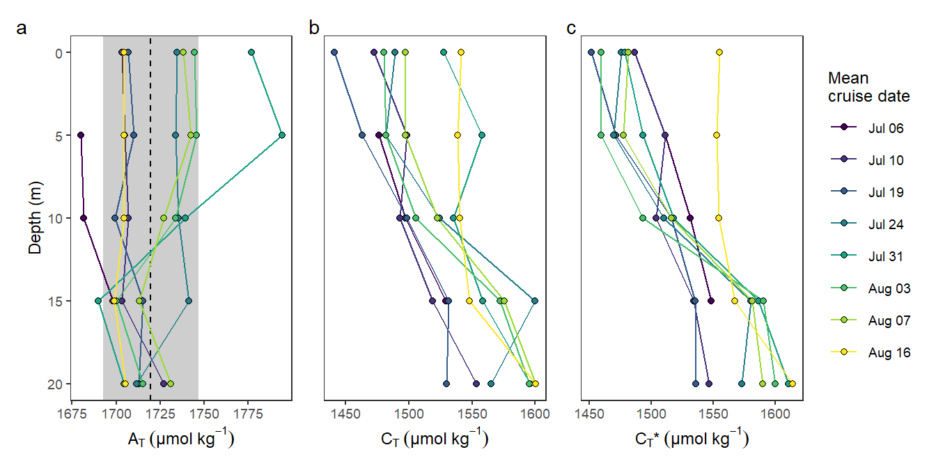
Discrete sample profiles as the mean of individual stations
ggsave(
  here::here(
    "output/Plots/Figures_publication/appendix",
    "Fig_B1.pdf"
  ),
  width = 160,
  height = 80,
  dpi = 300,
  units = "mm"
)

ggsave(
  here::here(
    "output/Plots/Figures_publication/appendix",
    "Fig_B1.png"
  ),
  width = 160,
  height = 80,
  dpi = 300,
  units = "mm"
)

rm(tb_long_mean, p_AT, p_CT, p_CT_star, tb_fix)
3.5 Surface time series
# surface time series per station
tb_surface <- tb_long %>%
  filter(dep < parameters$surface_dep) %>%
  group_by(ID, date_time_ID, var, station) %>%
  summarise(value = mean(value, na.rm = TRUE)) %>%
  ungroup()

# mean surface time series across stations
tb_surface_station_mean <- tb_long %>%
  filter(dep < parameters$surface_dep) %>%
  group_by(ID, date_time_ID, var) %>%
  summarise(value_mean = mean(value, na.rm = TRUE),
            value_sd = sd(value, na.rm = TRUE)) %>%
  ungroup()

# create time series plot
tb_long %>%
  filter(dep <= 10) %>%
  ggplot() +
  geom_line(data = tb_surface, aes(date_time_ID, value, col = "Individual")) +
  geom_line(data = tb_surface_station_mean, aes(date_time_ID, value_mean, col =
                                                  "Both (mean)")) +
  geom_point(aes(date_time_ID, value, fill = dep), shape = 21) +
  scale_fill_scico(palette = "oslo",
                   direction = -1,
                   name = "Depth (m)") +
  scale_color_brewer(palette = "Set1", name = "Station surface mean") +
  scale_x_datetime(breaks = "week", date_labels = "%d %b") +
  facet_grid(var ~ station, scales = "free_y") +
  labs(x = "Mean transect date")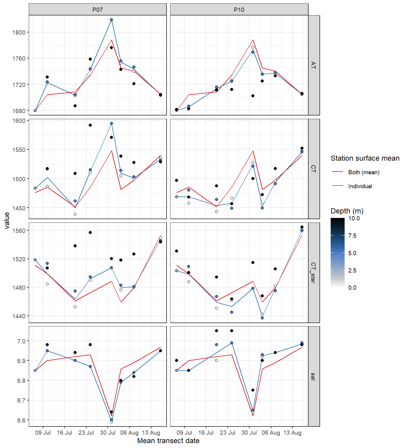
Time series of bottle data. Shown are raw data at water depth <= 10m, as well as mean values of samples collected at water depths < 6m (usually collected at 0 and 5 m).
rm(tb_long, tb_surface, tb)Note:
- CT* drop and temporal patterns agree well with those found in the CT* time series derived from pCO2 measurements (below).
4 CT* calculation from pCO2
Alkalinity normalized CT (CT*) profiles were calculated from sensor pCO2 and T profiles, and constant mean salinity and mean alkalinity values. Note that the impact of fixed vs. measured salinity has only a negligible impact on CT profiles.
# calculate CT_star for included profiles
tm_profiles <- tm_profiles %>%
  mutate(
    CT_star = carb(
      24,
      var1 = pCO2,
      var2 = AT_mean * 1e-6,
      S = sal_mean,
      T = tem,
      P = dep / 10,
      k1k2 = "m10",
      kf = "dg",
      ks = "d",
      gas = "insitu"
    )[, 16] * 1e6
  )

# calculate CT_star for excluded profiles
tm_profiles_stations_out <- tm_profiles_stations_out %>%
  drop_na() %>%
  mutate(
    CT_star = carb(
      24,
      var1 = pCO2,
      var2 = AT_mean * 1e-6,
      S = sal_mean,
      T = tem,
      P = dep / 10,
      k1k2 = "m10",
      kf = "dg",
      ks = "d",
      gas = "insitu"
    )[, 16] * 1e6
  )

# write CT_star profiles file
tm_profiles %>%
  write_csv(
    here::here(
      "data/intermediate/_merged_data_files/NCP_best_guess",
      "tm_profiles.csv"
    )
  )

# calculate CT_star test profiles for higher mean alkalinity
tm_profiles <- tm_profiles %>%
  mutate(
    CT_star_test = carb(
      24,
      var1 = pCO2,
      var2 = (AT_mean + 2*AT_sd) * 1e-6,
      S = sal_mean,
      T = tem,
      P = dep / 10,
      k1k2 = "m10",
      kf = "dg",
      ks = "d",
      gas = "insitu"
    )[, 16] * 1e6
  )
5 Profile plots
5.1 All individual profiles
# arrange by date (oldest first)
tm_profiles <-  tm_profiles %>%
  arrange(date_time_ID)

# create temperature profiles plots
p_tem <-
  tm_profiles %>%
  ggplot(aes(tem, dep, col = ID, group = interaction(station, ID))) +
  geom_path() +
  scale_y_reverse(expand = c(0, 0)) +
  labs(x = "Temp. (\u00B0C)",
       y = "Depth (m)") +
  scale_color_viridis_d(guide = FALSE) +
  theme(panel.grid.minor = element_blank())


# create pCO2 profiles plots
p_pCO2 <-
  tm_profiles %>%
  ggplot(aes(pCO2, dep, col = ID, group = interaction(station, ID))) +
  geom_path() +
  scale_y_reverse(expand = c(0, 0)) +
  labs(x = expression(italic(p)*CO[2] ~ (µatm))) +
  scale_color_viridis_d(guide = FALSE) +
  theme(
    axis.text.y = element_blank(),
    axis.title.y = element_blank(),
    axis.ticks.y = element_blank(),
    panel.grid.minor = element_blank()
  )

# create CT* profiles plots
p_CT_star <-
  tm_profiles %>%
  ggplot(aes(CT_star, dep, col = ID, group = interaction(station, ID))) +
  geom_path() +
  scale_y_reverse(expand = c(0, 0)) +
  scale_x_continuous(limits = c(1390, NA)) +
  labs(x = expression(paste(C[T], "*", ~ (µmol ~ kg ^ {-1})))) +
  scale_color_viridis_d(labels = cruise_dates$date_ID,
                        name = "Mean\ncruise date") +
  theme(
    axis.text.y = element_blank(),
    axis.ticks.y = element_blank(),
    axis.title.y = element_blank(),
    panel.grid.minor = element_blank()
  )


# Combine and safe plots to file
p_tem + p_pCO2 + p_CT_star +
  plot_annotation(tag_levels = 'a')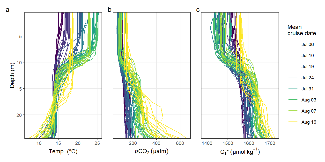
Individual vertical profiles per cruise day and station.
ggsave(
  here::here(
    "output/Plots/Figures_publication/article",
    "Fig_3.pdf"
  ),
  width = 160,
  height = 80,
  dpi = 300,
  units = "mm"
)

ggsave(
  here::here(
    "output/Plots/Figures_publication/article",
    "Fig_3.png"
  ),
  width = 160,
  height = 80,
  dpi = 300,
  units = "mm"
)

rm(p_tem, p_pCO2, p_CT_star)
5.2 Mean profiles
Mean vertical profiles were calculated for each cruise day (ID).
tm_profiles_ID_mean <- tm_profiles %>%
  select(-c(station, lat, lon, pCO2_corr, date_time)) %>%
  group_by(ID, date_time_ID, dep) %>%
  summarise_all(list(mean), na.rm = TRUE) %>%
  ungroup()

tm_profiles_ID_sd <- tm_profiles %>%
  select(-c(station, lat, lon, pCO2_corr, date_time)) %>%
  group_by(ID, date_time_ID, dep) %>%
  summarise_all(list(sd), na.rm = TRUE) %>%
  ungroup()

tm_profiles_ID_sd_long <- tm_profiles_ID_sd %>%
  pivot_longer(sal:CT_star_test, names_to = "var", values_to = "sd")

tm_profiles_ID_mean_long <- tm_profiles_ID_mean %>%
  pivot_longer(sal:CT_star_test, names_to = "var", values_to = "value")

tm_profiles_ID_long_test <-
  inner_join(tm_profiles_ID_mean_long, tm_profiles_ID_sd_long)

tm_profiles_ID_long <- tm_profiles_ID_long_test %>%
  filter(var != "CT_star_test")

tm_profiles_ID_mean_test <- tm_profiles_ID_mean

tm_profiles_ID_mean_test <- tm_profiles_ID_mean_test %>%
  mutate(CT_star_delta = CT_star - CT_star_test)

tm_profiles_ID_mean <- tm_profiles_ID_mean %>%
  select(-CT_star_test)

tm_profiles <- tm_profiles %>%
  select(-CT_star_test)

tm_profiles_ID_mean %>%
  write_csv(here::here("data/intermediate/_merged_data_files/NCP_best_guess", "tm_profiles_ID.csv"))

rm(
  tm_profiles_ID_sd_long,
  tm_profiles_ID_sd,
  tm_profiles_ID_mean_long
)
tm_profiles_ID_long %>%
ggplot(aes(value, dep, col = ID)) +
geom_point() +
geom_path() +
scale_y_reverse() +
scale_color_viridis_d() +
facet_wrap( ~ var, scales = "free_x")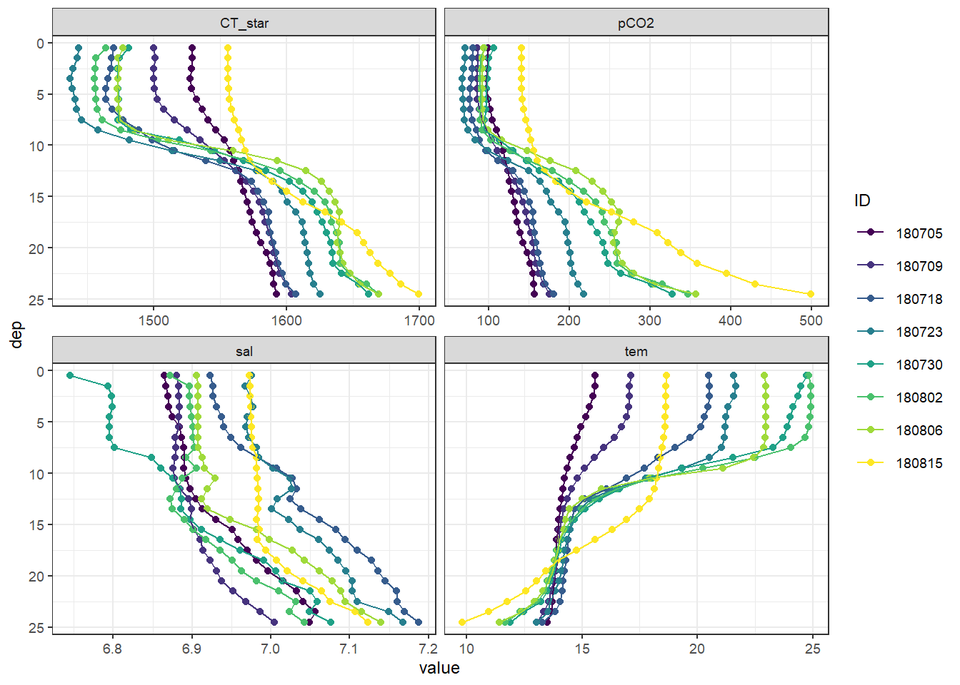
Mean vertical profiles per cruise day across all stations.
5.3 CT* sensitivity to mean AT
tm_profiles_ID_mean_test %>%
  ggplot(aes(CT_star_delta - mean(CT_star_delta), dep, col = ID)) +
  geom_point() +
  geom_path() +
  scale_y_reverse() +
  scale_color_viridis_d()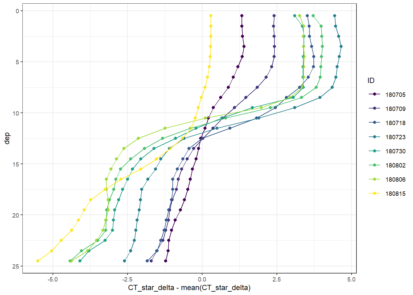
Offset between CT* calculate from mean AT and mean AT + 2 SD of AT, displayed as mean vertical profiles per cruise day across all stations.
5.4 All individual profiles per cruise day
profiles_min_max <- tm_profiles %>%
  group_by(dep) %>%
  summarise(max_CT = max(CT_star),
            min_CT = min(CT_star),
            max_tem = max(tem),
            min_tem = min(tem)) %>%
  ungroup()

p_CT_star <-
  tm_profiles %>%
  ggplot() +
  geom_ribbon(data = profiles_min_max,
              aes(xmin = min_CT,
                  xmax = max_CT,
                  y = dep),
              alpha = 0.2) +
   geom_path(aes(CT_star, dep, col = station)) +
  scale_y_reverse() +
  facet_grid(ID ~ .) +
  labs(x = expression(paste(C[T], "*", ~ (µmol ~ kg ^ {-1}))),
  y = "Depth (m)") +
  theme(strip.background = element_blank(),
        strip.text = element_blank(),
        legend.position = "none",
        panel.grid.minor = element_blank())

cruise_labels <- c(
  `180705` = cruise_dates$date_ID[1],
  `180709` = cruise_dates$date_ID[2],
  `180718` = cruise_dates$date_ID[3],
  `180723` = cruise_dates$date_ID[4],
  `180730` = cruise_dates$date_ID[5],
  `180802` = cruise_dates$date_ID[6],
  `180806` = cruise_dates$date_ID[7],
  `180815` = cruise_dates$date_ID[8]
)

p_tem <-
  tm_profiles %>%
  ggplot() +
  geom_ribbon(data = profiles_min_max,
              aes(xmin = min_tem,
                  xmax = max_tem,
                  y = dep,
                  fill = "Min/Max"),
              alpha = 0.2) +
  geom_path(aes(tem, dep, col = station)) +
  scale_y_reverse() +
  scale_fill_manual(values = "black", name = "") +
  scale_color_discrete(name = "Station") +
  guides(color = guide_legend(order = 1)) +
  facet_grid(ID ~ .,
             labeller = labeller(ID = cruise_labels)) +
  labs(x = "Temperature (\u00B0C)",
       y = "Depth (m)") +
  theme(axis.title.y = element_blank(),
        axis.text.y = element_blank(),
        axis.ticks.y = element_blank(),
        panel.grid.minor = element_blank())

p_CT_star | p_tem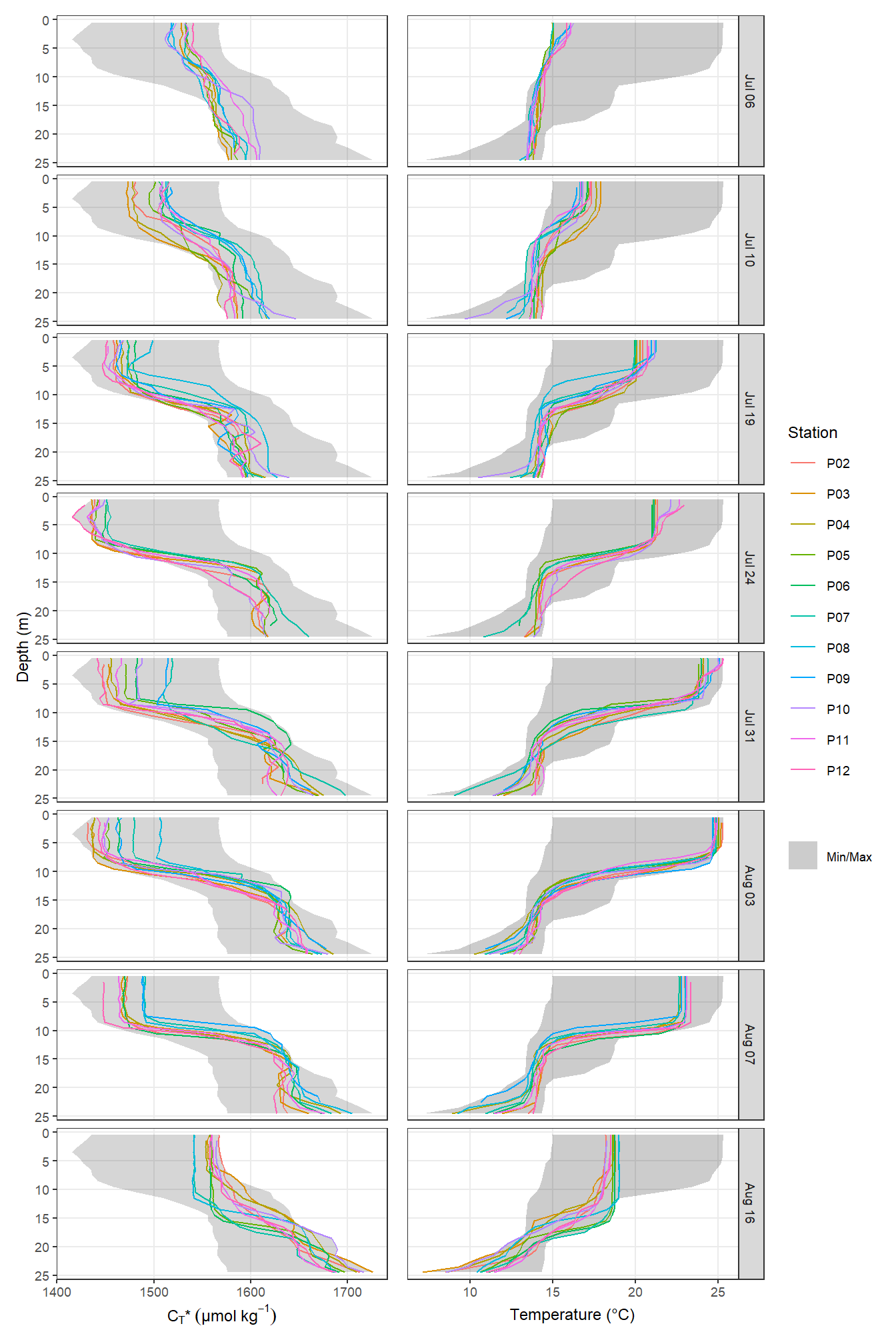
Mean vertical profiles per cruise day across all stations plotted indivdually. Ribbons indicate the standard deviation observed across all profiles at each depth and transect.
ggsave(
  here::here(
    "output/Plots/Figures_publication/appendix",
    "Fig_C3.pdf"
  ),
  width = 120,
  height = 180,
  dpi = 300,
  units = "mm"
)

ggsave(
  here::here(
    "output/Plots/Figures_publication/appendix",
    "Fig_C3.png"
  ),
  width = 120,
  height = 180,
  dpi = 300,
  units = "mm"
)

rm(p_CT_star, p_tem, cruise_labels, profiles_min_max)
Important notes:
- the standard deviation of CT in the upper 10m increases on June 30.
CT, pCO2, S, and T profiles were plotted individually pdf here and grouped by ID pdf here. The later gives an idea of the differences between stations at one point in time.
# create pdf file
pdf(file=here::here("output/Plots/NCP_best_guess",
    "tm_profiles_pCO2_tem_sal_CT.pdf"), onefile = TRUE, width = 9, height = 5)

# loop across all stations and cruise days and create profile plots
for(i_ID in unique(tm_profiles$ID)){
  for(i_station in unique(tm_profiles$station)){

    if (nrow(tm_profiles %>% filter(ID == i_ID, station == i_station)) > 0){

      # i_ID      <-      unique(tm_profiles$ID)[1]
      # i_station <- unique(tm_profiles$station)[1]

      p_pCO2 <-
        tm_profiles %>%
        arrange(date_time) %>%
        filter(ID == i_ID,
               station == i_station) %>%
        ggplot(aes(pCO2, dep, col="grid_RT"))+
        geom_point(aes(pCO2_corr, dep, col="grid"))+
        geom_point()+
        geom_path()+
        scale_y_reverse()+
        scale_color_brewer(palette = "Set1")+
        labs(y="Depth [m]", x="pCO2 [µatm]", title = str_c(i_ID," | ",i_station))+
        coord_cartesian(xlim = c(0,200), ylim = c(30,0))+
        theme_bw()+
        theme(legend.position = "left")

      p_tem <-
        tm_profiles %>%
        arrange(date_time) %>%
        filter(ID == i_ID,
               station == i_station) %>%
        ggplot(aes(tem, dep))+
        geom_point()+
        geom_path()+
        scale_y_reverse()+
        labs(y="Depth [m]", x="Tem [°C]")+
        coord_cartesian(xlim = c(14,26), ylim = c(30,0))+
        theme_bw()

      p_sal <-
        tm_profiles %>%
        arrange(date_time) %>%
        filter(ID == i_ID,
               station == i_station) %>%
        ggplot(aes(sal, dep))+
        geom_point()+
        geom_path()+
        scale_y_reverse()+
        labs(y="Depth [m]", x="Tem [°C]")+
        coord_cartesian(xlim = c(6.5,7.5), ylim = c(30,0))+
        theme_bw()

      p_CT_star <-
        tm_profiles %>%
        arrange(date_time) %>%
        filter(ID == i_ID,
               station == i_station) %>%
        ggplot(aes(CT_star, dep))+
        geom_point()+
        geom_path()+
        scale_y_reverse()+
        labs(y="Depth [m]", x="CT_star* [µmol/kg]")+
        coord_cartesian(xlim = c(1400,1700), ylim = c(30,0))+
        theme_bw()


      print(
            p_pCO2 + p_tem + p_sal + p_CT_star
            )

      rm(p_pCO2, p_sal, p_tem, p_CT_star)


    }
  }
}

dev.off()

rm(i_ID, i_station)
# convert data to long format
tm_profiles_long <- tm_profiles %>%
select(-c(lat, lon, pCO2_corr)) %>%
pivot_longer(sal:CT_star, values_to = "value", names_to = "var")
# create pdf file
pdf(file=here::here("output/Plots/NCP_best_guess",
"tm_profiles_ID_pCO2_tem_sal_CT.pdf"), onefile = TRUE, width = 9, height = 5)
# loop across all cruise days and create profile plots
for(i_ID in unique(tm_profiles$ID)){
#i_ID <- unique(tm_profiles$ID)[1]
sub_tm_profiles_long <- tm_profiles_long %>%
arrange(date_time) %>%
filter(ID == i_ID)
print(
sub_tm_profiles_long %>%
ggplot()+
geom_path(data = tm_profiles_long,
aes(value, dep, group=interaction(station, ID)), col="grey")+
geom_path(aes(value, dep, col=station))+
scale_y_reverse()+
labs(y="Depth [m]", title = str_c("ID: ", i_ID))+
theme_bw()+
facet_wrap(~var, scales = "free_x")
)
rm(sub_tm_profiles_long)
}
dev.off()
rm(i_ID, tm_profiles_long)5.5 All excluded individual profiles per cruise day
# calculate overall min/max profiles from included stations
profiles_min_max <- tm_profiles %>%
  group_by(dep, ID) %>%
  summarise(max_CT = max(CT_star),
            min_CT = min(CT_star),
            max_tem = max(tem),
            min_tem = min(tem)) %>%
  ungroup()

# calculate overall mean +/- SD profiles from included stations
profiles_sd <- tm_profiles %>%
  group_by(dep, ID) %>%
  summarise(max_CT = mean(CT_star) + sd(CT_star),
            min_CT = mean(CT_star) - sd(CT_star),
            max_tem = mean(tem) + sd(tem),
            min_tem = mean(tem) - sd(tem)) %>%
  ungroup()

# filter downcast from relevant excluded stations
tm_profiles_stations_out <- tm_profiles_stations_out %>%
  filter(ID %in% unique(tm_profiles$ID),
         phase == "down")

# plot profiles
p_CT <-
  tm_profiles_stations_out %>%
  ggplot() +
  geom_ribbon(data = profiles_min_max,
              aes(xmin = min_CT,
                  xmax = max_CT,
                  y = dep,
                  fill = "Min/Max"),
              alpha = 0.2) +
  geom_ribbon(data = profiles_sd,
              aes(xmin = min_CT,
                  xmax = max_CT,
                  y = dep,
                  fill = "SD"),
              alpha = 0.2) +
  scale_fill_manual(values = c("black", "purple"), name = "") +
  geom_path(aes(CT_star, dep, col = station)) +
  scale_y_reverse() +
  facet_grid(ID ~ .) +
  labs(x = expression(paste(C[T], "*", ~ (µmol ~ kg ^ {
    -1
  }))),
  y = "Depth (m)") +
  theme(
    strip.background = element_blank(),
    strip.text = element_blank(),
    legend.position = "none"
  )

cruise_labels <- c(
  `180705` = cruise_dates$date_ID[1],
  `180709` = cruise_dates$date_ID[2],
  `180718` = cruise_dates$date_ID[3],
  `180723` = cruise_dates$date_ID[4],
  `180730` = cruise_dates$date_ID[5],
  `180802` = cruise_dates$date_ID[6],
  `180806` = cruise_dates$date_ID[7],
  `180815` = cruise_dates$date_ID[8]
)

p_tem <-
  tm_profiles_stations_out %>%
  ggplot() +
  geom_ribbon(data = profiles_min_max,
              aes(xmin = min_tem,
                  xmax = max_tem,
                  y = dep,
                  fill = "Min/Max"),
              alpha = 0.2) +
  geom_ribbon(data = profiles_sd,
              aes(xmin = min_tem,
                  xmax = max_tem,
                  y = dep,
                  fill = "SD"),
              alpha = 0.2) +
  geom_path(aes(tem, dep, col = station)) +
  scale_y_reverse() +
  scale_fill_manual(values = c("black", "purple"), name = "") +
  scale_color_discrete(name = "Station") +
  guides(color = guide_legend(order = 1)) +
  facet_grid(ID ~ .,
             labeller = labeller(ID = cruise_labels)) +
  labs(x = "Temperature (\u00B0C)",
       y = "Depth (m)") +
  theme(axis.title.y = element_blank(),
        axis.text.y = element_blank())

p_CT | p_tem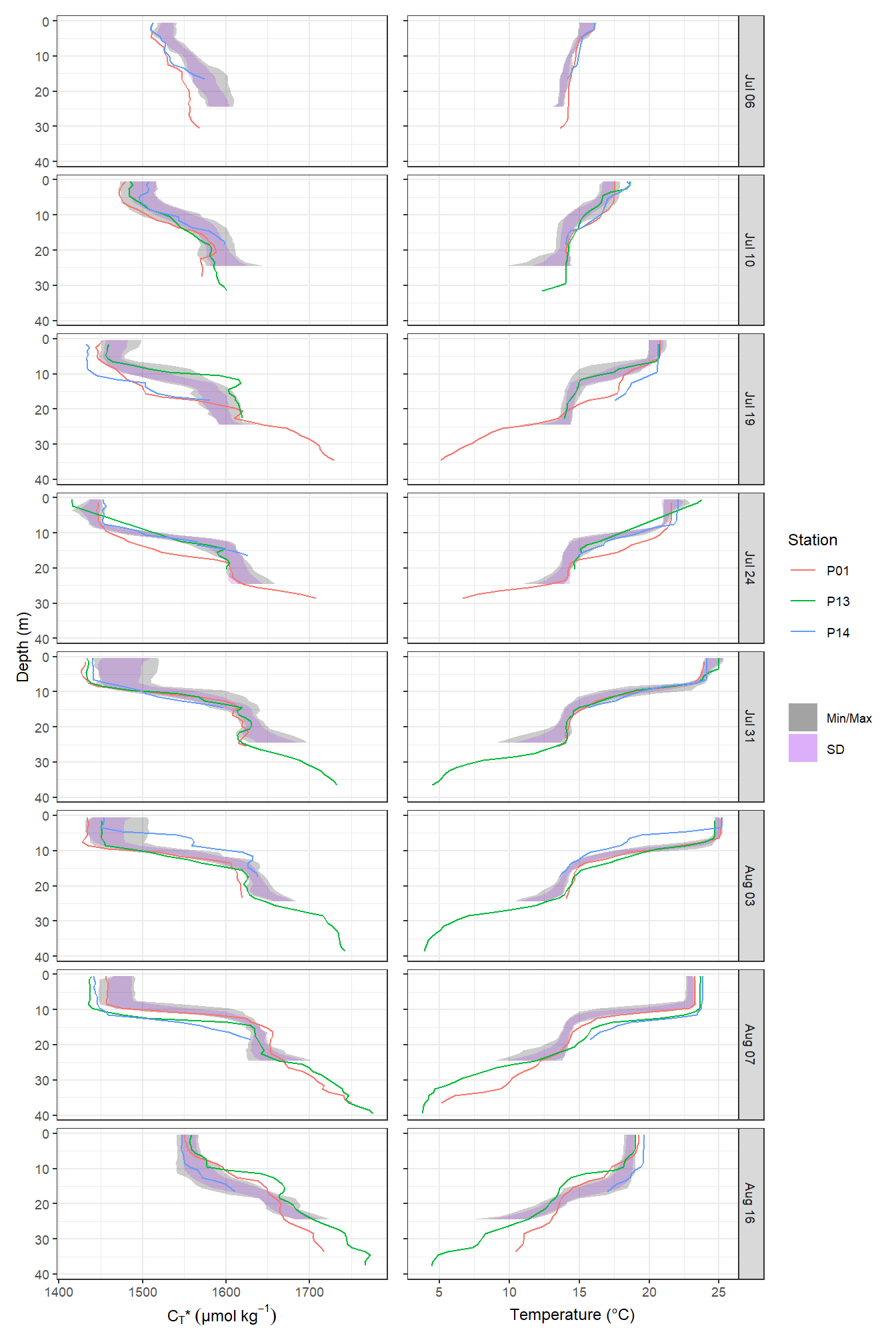
Mean vertical profiles per cruise day across all stations plotted indivdually. Ribbons indicate the standard deviation observed across all profiles at each depth and transect.
rm(p_CT_star, p_tem, cruise_labels, profiles_min_max,
   profiles_sd, p_CT)
5.6 Incremental changes
Changes of seawater variables at each depth are calculated from one cruise day to the next and divided by the number of days inbetween.
tm_profiles_ID_long <- tm_profiles_ID_long %>%
  group_by(var, dep) %>%
  arrange(date_time_ID) %>%
  mutate(
    date_time_ID_diff = as.numeric(date_time_ID - lag(date_time_ID)),
    date_time_ID_ref  = date_time_ID - (date_time_ID - lag(date_time_ID)) /
      2,
    value_diff = value     - lag(value, default = first(value)),
    value_diff_daily = value_diff / date_time_ID_diff,
    value_cum = cumsum(value_diff)
  ) %>%
  ungroup()
tm_profiles_ID_long %>%
arrange(dep) %>%
ggplot(aes(value_diff_daily, dep, col = ID)) +
geom_vline(xintercept = 0) +
geom_point() +
geom_path() +
scale_y_reverse() +
scale_color_viridis_d() +
facet_wrap( ~ var, scales = "free_x") +
labs(x = "Change of value inbetween cruises per day")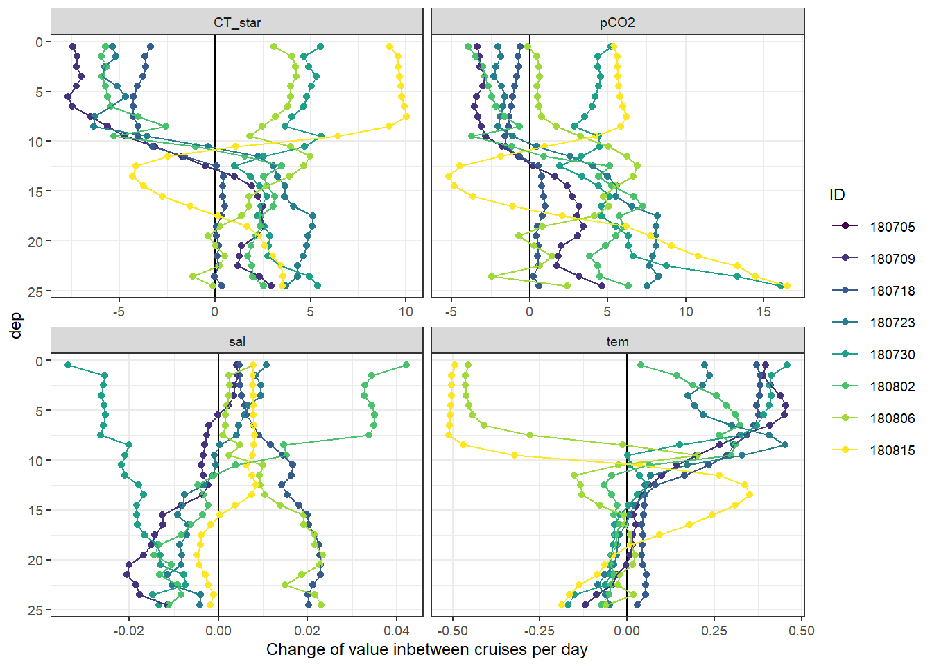
5.7 Cumulative changes
Cumulative changes of seawater vars were calculated at each depth relative to the first cruise day on July 5.
tm_profiles_ID_long %>%
  arrange(dep) %>%
  ggplot(aes(value_cum, dep, col = ID)) +
  geom_vline(xintercept = 0) +
  geom_point() +
  geom_path() +
  scale_y_reverse() +
  scale_color_viridis_d() +
  facet_wrap( ~ var, scales = "free_x") +
  labs(x = "Cumulative change of value")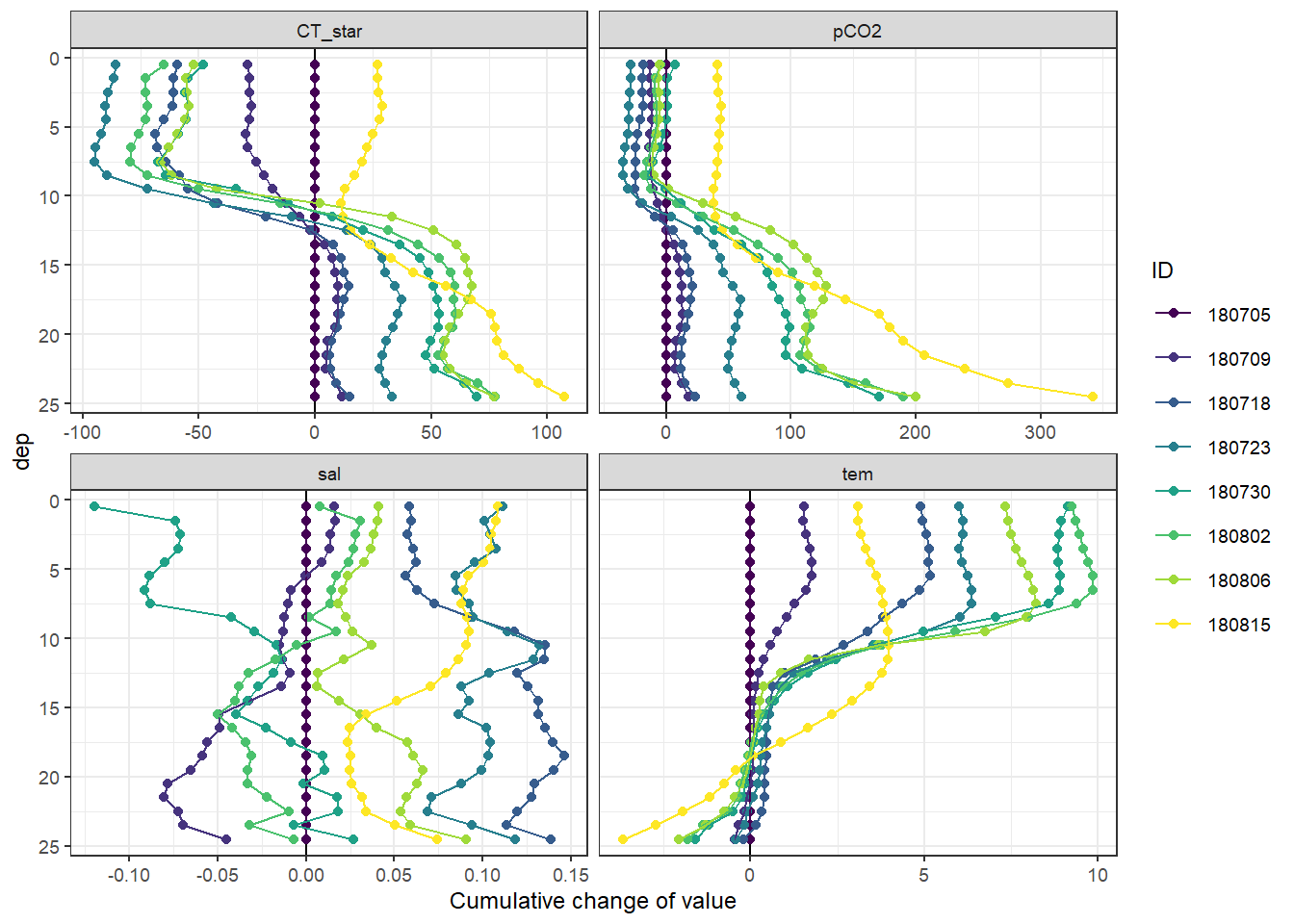
Important notes:
- Salinity in the upper 10m decreases by >0.1 on June 30, and returns to average conditions already on Aug 02.
5.8 Cumulative changes by sign
Cumulative positive and negative changes of seawater vars were calculated separately at each depth relative to the first cruise day on July 5.
tm_profiles_ID_long <- tm_profiles_ID_long %>%
  mutate(sign = if_else(value_diff < 0, "neg", "pos")) %>%
  group_by(var, dep, sign) %>%
  arrange(date_time_ID) %>%
  mutate(value_cum_sign = cumsum(value_diff)) %>%
  ungroup()
tm_profiles_ID_long %>%
arrange(dep) %>%
ggplot(aes(value_cum_sign, dep, col = ID)) +
geom_vline(xintercept = 0) +
geom_point() +
geom_path() +
scale_y_reverse() +
scale_color_viridis_d() +
scale_fill_viridis_d() +
facet_wrap( ~ interaction(sign, var), scales = "free_x", ncol = 4) +
labs(x = "Cumulative directional change of value")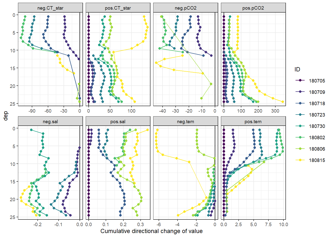
6 Time series plots
6.1 Depth intervals
Mean seawater parameters were calculated for 5m depth intervals.
# cut into 5m depth intervals
tm_profiles_ID_long_grid <- tm_profiles_ID_long %>%
  mutate(dep = cut(dep, seq(0, 30, 5))) %>%
  group_by(ID, date_time_ID, dep, var)  %>%
  summarise_all(list(mean), na.rm = TRUE) %>%
  ungroup()

tm_profiles_ID_long_grid %>%
  ggplot(aes(date_time_ID, value, col = as.factor(dep))) +
  geom_path() +
  geom_point() +
  scale_color_viridis_d(name = "Depth (m)") +
  scale_x_datetime(breaks = "week", date_labels = "%d %b") +
  facet_wrap( ~ var, scales = "free_y", ncol = 1) +
  theme(axis.title.x = element_blank())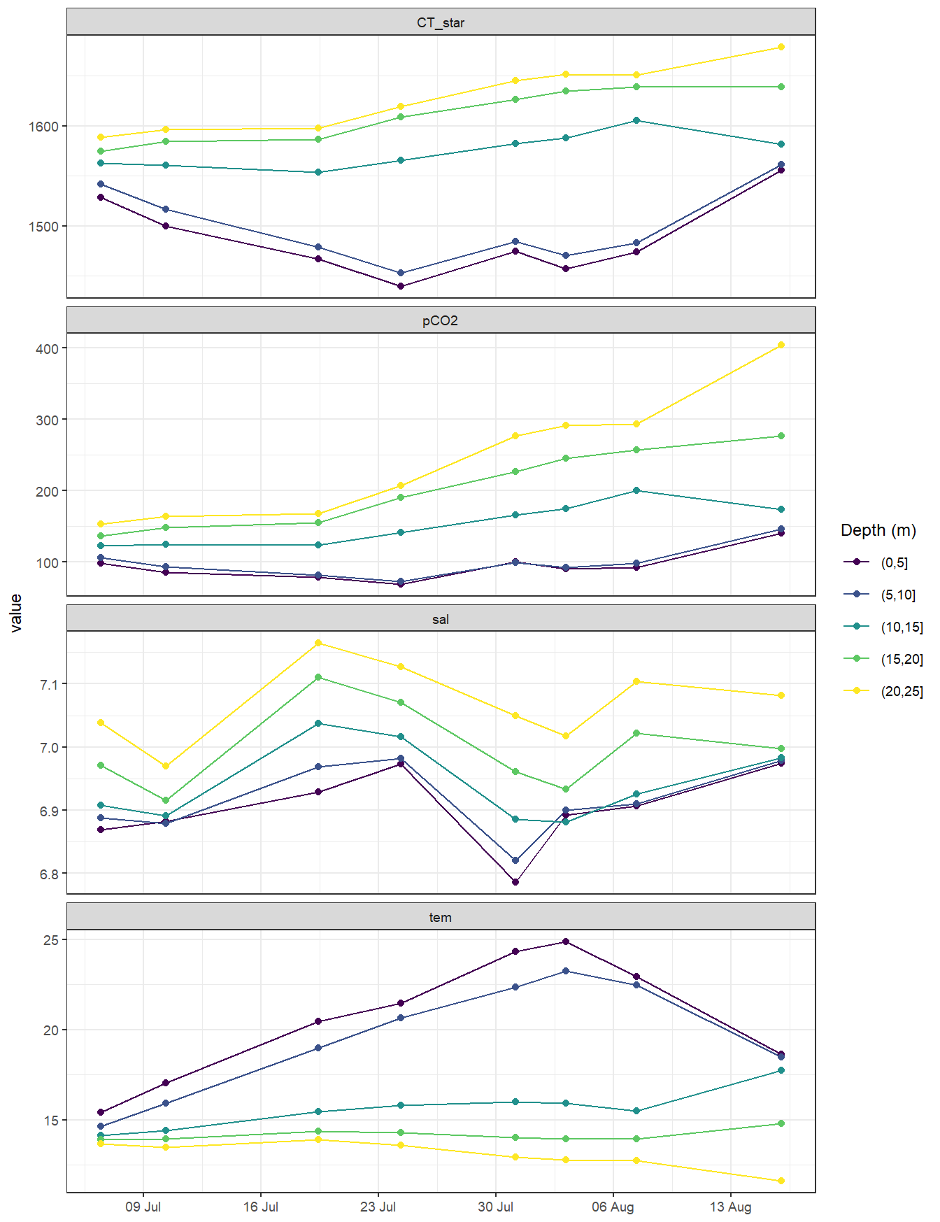
tm_profiles_ID_long_grid %>%
  mutate(value = round(value, 1),
         date_ID = as.Date(date_time_ID)) %>%
  select(date_ID, dep, var, value) %>%
  pivot_wider(values_from = value, names_from = var) %>%
  kable() %>%
  add_header_above() %>%
  kable_styling(full_width = FALSE) %>%
scroll_box(height = "400px")| date_ID | dep | CT_star | pCO2 | sal | tem |
|---|---|---|---|---|---|
| 2018-07-06 | (0,5] | 1528.4 | 98.3 | 6.9 | 15.4 |
| 2018-07-06 | (5,10] | 1541.9 | 106.0 | 6.9 | 14.7 |
| 2018-07-06 | (10,15] | 1562.9 | 123.3 | 6.9 | 14.1 |
| 2018-07-06 | (15,20] | 1575.1 | 136.5 | 7.0 | 13.9 |
| 2018-07-06 | (20,25] | 1589.1 | 153.4 | 7.0 | 13.7 |
| 2018-07-10 | (0,5] | 1500.2 | 86.0 | 6.9 | 17.0 |
| 2018-07-10 | (5,10] | 1517.0 | 93.4 | 6.9 | 15.9 |
| 2018-07-10 | (10,15] | 1561.0 | 124.7 | 6.9 | 14.4 |
| 2018-07-10 | (15,20] | 1584.4 | 148.5 | 6.9 | 14.0 |
| 2018-07-10 | (20,25] | 1596.2 | 163.9 | 7.0 | 13.5 |
| 2018-07-19 | (0,5] | 1466.8 | 79.1 | 6.9 | 20.5 |
| 2018-07-19 | (5,10] | 1479.3 | 81.5 | 7.0 | 19.0 |
| 2018-07-19 | (10,15] | 1553.9 | 124.4 | 7.0 | 15.5 |
| 2018-07-19 | (15,20] | 1586.9 | 155.0 | 7.1 | 14.4 |
| 2018-07-19 | (20,25] | 1597.8 | 168.3 | 7.2 | 13.9 |
| 2018-07-24 | (0,5] | 1440.0 | 69.1 | 7.0 | 21.5 |
| 2018-07-24 | (5,10] | 1453.4 | 73.2 | 7.0 | 20.7 |
| 2018-07-24 | (10,15] | 1565.5 | 141.8 | 7.0 | 15.8 |
| 2018-07-24 | (15,20] | 1609.3 | 190.8 | 7.1 | 14.3 |
| 2018-07-24 | (20,25] | 1619.2 | 207.1 | 7.1 | 13.6 |
| 2018-07-31 | (0,5] | 1474.7 | 100.3 | 6.8 | 24.3 |
| 2018-07-31 | (5,10] | 1484.4 | 99.2 | 6.8 | 22.3 |
| 2018-07-31 | (10,15] | 1582.6 | 165.6 | 6.9 | 16.0 |
| 2018-07-31 | (15,20] | 1626.7 | 226.6 | 7.0 | 14.0 |
| 2018-07-31 | (20,25] | 1645.6 | 277.0 | 7.0 | 12.9 |
| 2018-08-03 | (0,5] | 1457.3 | 90.7 | 6.9 | 24.9 |
| 2018-08-03 | (5,10] | 1470.6 | 92.8 | 6.9 | 23.3 |
| 2018-08-03 | (10,15] | 1588.2 | 174.5 | 6.9 | 15.9 |
| 2018-08-03 | (15,20] | 1634.7 | 245.5 | 6.9 | 13.9 |
| 2018-08-03 | (20,25] | 1651.7 | 291.4 | 7.0 | 12.8 |
| 2018-08-07 | (0,5] | 1473.8 | 92.4 | 6.9 | 23.0 |
| 2018-08-07 | (5,10] | 1483.4 | 98.6 | 6.9 | 22.5 |
| 2018-08-07 | (10,15] | 1605.2 | 200.1 | 6.9 | 15.5 |
| 2018-08-07 | (15,20] | 1638.8 | 257.3 | 7.0 | 14.0 |
| 2018-08-07 | (20,25] | 1651.3 | 293.4 | 7.1 | 12.7 |
| 2018-08-16 | (0,5] | 1556.0 | 140.7 | 7.0 | 18.6 |
| 2018-08-16 | (5,10] | 1561.3 | 146.8 | 7.0 | 18.5 |
| 2018-08-16 | (10,15] | 1581.8 | 173.5 | 7.0 | 17.7 |
| 2018-08-16 | (15,20] | 1638.9 | 276.9 | 7.0 | 14.8 |
| 2018-08-16 | (20,25] | 1679.2 | 404.0 | 7.1 | 11.6 |
rm(tm_profiles_ID_long_grid)7 CT* sensitivity to mean AT
Mean seawater CT* were calculated for 5m depth intervals, based on two AT values (regular mean + 2 SD). Relative changes of CT* do not differ much, despite a large bias in mean AT.
# cut into 5m depth intervals
tm_profiles_ID_long_grid <- tm_profiles_ID_long_test %>%
  mutate(dep = cut(dep, seq(0, 30, 5))) %>%
  group_by(ID, date_time_ID, dep, var)  %>%
  summarise_all(list(mean), na.rm = TRUE)

tm_profiles_ID_long_grid %>%
  filter(var %in% c("CT_star", "CT_star_test")) %>%
  ggplot(aes(date_time_ID, value, col = as.factor(dep))) +
  geom_path() +
  geom_point() +
  scale_color_viridis_d(name = "Depth (m)") +
  scale_x_datetime(breaks = "week", date_labels = "%d %b") +
  facet_wrap( ~ var, scales = "free_y", ncol = 1) +
  theme(axis.title.x = element_blank())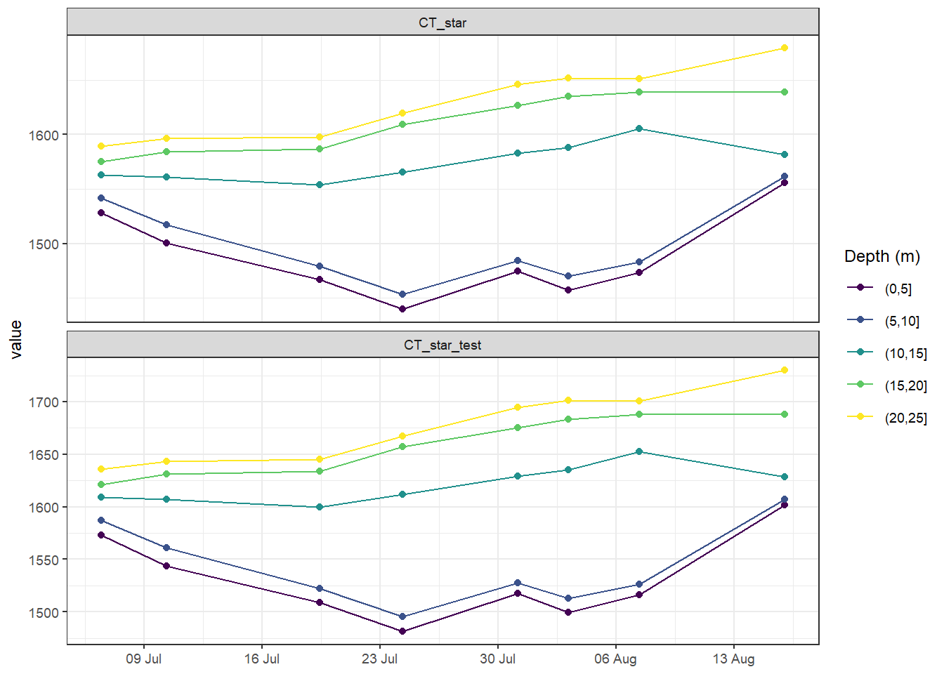
rm(tm_profiles_ID_long_grid, tm_profiles_ID_long_test)To further illustrate the robustness of CT* to errors in mean AT, we calculate CT* changes for range of AT errors and the conditions encountered during the field campaign in 2018.
# prepare data set with peak values of cyano bloom
CT_star_sens <- tm_profiles %>%
  filter(dep < parameters$surface_dep,
         date_ID %in% c("Jul 06", "Jul 24")) %>%
  select(date_ID, tem, pCO2) %>%
  group_by(date_ID) %>%
  summarise_all(mean, na.rm = TRUE) %>%
  ungroup()

# create range of AT values spanning +/- 3 SD
CT_star_sens <- expand_grid(CT_star_sens, factor = seq(-3, 3, 0.2))

CT_star_sens <- CT_star_sens %>%
  mutate(AT = (AT_mean + factor * AT_sd) * 1e-6)

# calculate C* for range of AT values
CT_star_sens <- CT_star_sens %>%
  mutate(
    CT_star = carb(
      24,
      var1 = pCO2,
      var2 = AT,
      S = sal_mean,
      T = tem,
      k1k2 = "m10",
      kf = "dg",
      ks = "d",
      gas = "insitu"
    )[, 16] * 1e6
  )

# calculate change of CT* for various AT values
CT_star_sens <- CT_star_sens %>%
  mutate(AT = AT * 1e6) %>%
  select(date_ID, factor, AT, CT_star) %>%
  pivot_wider(names_from = "date_ID",
              values_from = c("CT_star"))

CT_star_sens <- CT_star_sens %>%
  mutate(CT_star_delta = `Jul 24` - `Jul 06`) %>%
  select(factor, AT, CT_star_delta)

CT_star_delta_mean <- CT_star_sens %>%
  filter(factor == 0) %>%
  pull(CT_star_delta)

CT_star_sens <- CT_star_sens %>%
  mutate(
    CT_star_delta_offset = CT_star_delta - CT_star_delta_mean,
    CT_star_delta_offset_rel = CT_star_delta / CT_star_delta_mean * 100,
    AT_offset = AT - AT_mean
  )

CT_star_delta_sd <- CT_star_sens %>%
  filter(factor == 1) %>%
  pull(CT_star_delta_offset)


CT_star_sens %>%
  ggplot(aes(AT_offset, CT_star_delta_offset)) +
  annotate(
    "rect",
    xmin = -AT_sd,
    xmax = +AT_sd,
    ymin = -Inf,
    ymax = Inf,
    alpha = 0.3
  ) +
  annotate(
    "rect",
    xmin = -Inf,
    xmax = Inf,
    ymin = -CT_star_delta_sd,
    ymax = +CT_star_delta_sd,
    alpha = 0.3
  ) +
  geom_vline(xintercept = 0, linetype = 2) +
  geom_hline(yintercept = 0, linetype = 2) +
  geom_line(col = "red") +
  scale_y_continuous(
    expression(paste(
      "Absolute bias ", Delta ~ C[T], "*",  ~ (µmol ~ kg ^ {
        -1
      })
    )),
    sec.axis = sec_axis(
      ~ . / CT_star_delta_mean * 100,
      name = expression(paste("Relative bias ", Delta ~ C[T], "* (%)")),
      breaks = seq(-10, 10, 1)
    )
  ) +
  scale_x_continuous(expression(paste("Absolute bias ", A[T]  ~ (µmol ~ kg ^ {
    -1
  }))),
  sec.axis = sec_axis(
    ~ . / AT_mean * 100,
    name = expression(paste("Relative bias ", A[T], " (%)")),
    breaks = seq(-10, 10, 1)
  )) +
  theme(panel.grid = element_blank())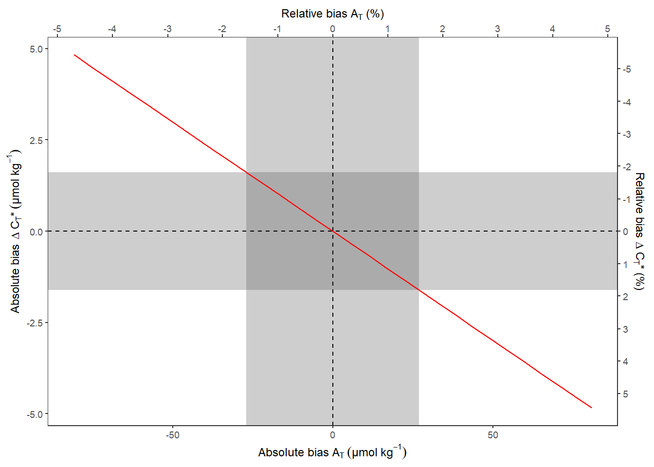
ggsave(
  here::here("output/Plots/Figures_publication/appendix",
             "Fig_C1.pdf"),
  width = 83,
  height = 60,
  dpi = 300,
  units = "mm"
)

ggsave(
  here::here("output/Plots/Figures_publication/appendix",
             "Fig_C1.png"),
  width = 83,
  height = 60,
  dpi = 300,
  units = "mm"
)

rm(CT_star_delta_mean, CT_star_delta_sd,
   CT_star_sens)
8 Hovmoeller plots
8.1 Absolute values
bin_CT_star <- 30

grid_raster <- expand_grid(cruise_dates,
                      dep = seq(5,20,5))

p_CT_star_hov <-
  tm_profiles_ID_long %>%
  filter(var == "CT_star") %>%
  ggplot() +
  geom_contour_fill(aes(x = date_time_ID, y = dep, z = value),
                    breaks = MakeBreaks(bin_CT_star),
                    col = "black",
                    size = 0.1) +
  geom_point(data = grid_raster,
             aes(date_time_ID, dep),
             col = "white",
             shape = 3,
             size = 0.7) +
  scale_fill_scico(
    breaks = MakeBreaks(bin_CT_star),
    guide = "colorstrip",
    name = expression(paste(C[T],"*")~(µmol ~ kg ^ {-1})~" "),
    palette = "davos",
    direction = -1
  ) +
  guides(fill = guide_colorsteps(barheight = unit(3, "mm"),
                                 barwidth = unit(65, "mm"),
                                 frame.colour = "black",
                                 ticks = TRUE,
                                 ticks.colour = "black")) +
  scale_y_reverse() +
  scale_x_datetime(breaks = "week",
                   date_labels = "%b %d") +
  labs(y = "Depth (m)") +
  coord_cartesian(expand = 0) +
  theme(
    axis.title.x = element_blank(),
    legend.position = "bottom",
    legend.margin = margin(0, 0, 0, 0),
    legend.box.margin = margin(0, 0, 0, 0)
  )

bin_Tem <- 2

p_tem_hov <- tm_profiles_ID_long %>%
  filter(var == "tem") %>%
  ggplot() +
  geom_contour_fill(aes(x = date_time_ID, y = dep, z = value),
                    breaks = MakeBreaks(bin_Tem),
                    col = "black",
                    size = 0.1) +
  geom_point(data = grid_raster,
             aes(date_time_ID, dep),
             col = "white",
             shape = 3,
             size = 0.7) +
  scale_fill_viridis_c(
    breaks = MakeBreaks(bin_Tem),
    guide = "colorstrip",
    name = expression(Temp.~("\u00B0" * C)),
    option = "inferno"
  ) +
  guides(fill = guide_colorsteps(barheight = unit(3, "mm"),
                                 barwidth = unit(55, "mm"),
                                 frame.colour = "black",
                                 ticks = TRUE,
                                 ticks.colour = "black")) +
  scale_y_reverse() +
  scale_x_datetime(breaks = "week",
                   date_labels = "%b %d") +
  labs(y = "Depth (m)") +
  coord_cartesian(expand = 0) +
  theme(
    axis.title.x = element_blank(),
    legend.position = "top",
    legend.margin = margin(0, 0, 0, 0),
    legend.box.margin = margin(0, 0, 0, 0)
  )

cum_cruise_dates <- cruise_dates %>% filter(ID != "180705")
viridis_cum_cruise_dates <- hcl.colors(nrow(cruise_dates))[2:8]

p_CT_star_ID_cum <-
  tm_profiles_ID_long %>%
  filter(var == "CT_star",
         ID != "180705") %>%
  ggplot(aes(value_cum, dep, col = ID, fill = ID)) +
  geom_hline(yintercept = 12, col = "red") +
  geom_vline(xintercept = 0) +
  geom_path() +
  geom_point(shape = 21, col = "black") +
  scale_y_reverse(expand = c(0, 0),
                  position = "right") +
  labs(x = expression(paste(Delta~C[T],"*", ~ cumulative ~ (µmol ~ kg ^ {
    -1
  }))),
  y = "Depth (m)") +
  scale_color_viridis_d(labels = cum_cruise_dates$date_ID, guide = FALSE) +
  scale_fill_viridis_d(labels = cum_cruise_dates$date_ID, guide = FALSE) +
  # scale_color_manual(values = viridis_cum_cruise_dates,
  #                    labels = cum_cruise_dates$date_ID,
  #                    guide = FALSE) +
  # scale_fill_manual(values = viridis_cum_cruise_dates,
  #                   labels = cum_cruise_dates$date_ID,
  #                   guide = FALSE) +
  theme(panel.grid.minor = element_blank())

p_tem_ID_cum <-
  tm_profiles_ID_long %>%
  filter(var == "tem",
         ID != "180705") %>%
  ggplot(aes(value_cum, dep, col = ID, fill = ID)) +
  geom_hline(yintercept = 12, col = "red") +
  geom_vline(xintercept = 0) +
  geom_path() +
  geom_point(shape = 21, col = "black") +
  scale_y_reverse(expand = c(0, 0),
                  position = "right") +
  labs(x = expression(Delta~"Temp. cumulative (\u00B0C)"),
       y = "Depth (m)") +
  scale_color_manual(values = viridis_cum_cruise_dates,
                     labels = cum_cruise_dates$date_ID) +
  scale_fill_manual(values = viridis_cum_cruise_dates,
                     labels = cum_cruise_dates$date_ID) +
  theme(
    legend.position = "top",
    legend.title = element_blank(),
    legend.key.size = unit(4, "mm"),
    legend.key.width = unit(4,"mm"),
    panel.grid.minor = element_blank()
  )

((p_tem_hov | p_tem_ID_cum ) + plot_layout(tag_level = 'new', widths = c(2.3, 1))) /
((p_CT_star_hov | p_CT_star_ID_cum ) + plot_layout(tag_level = 'new', widths = c(2.3, 1))) +
  plot_annotation(tag_levels = c('a', '1'))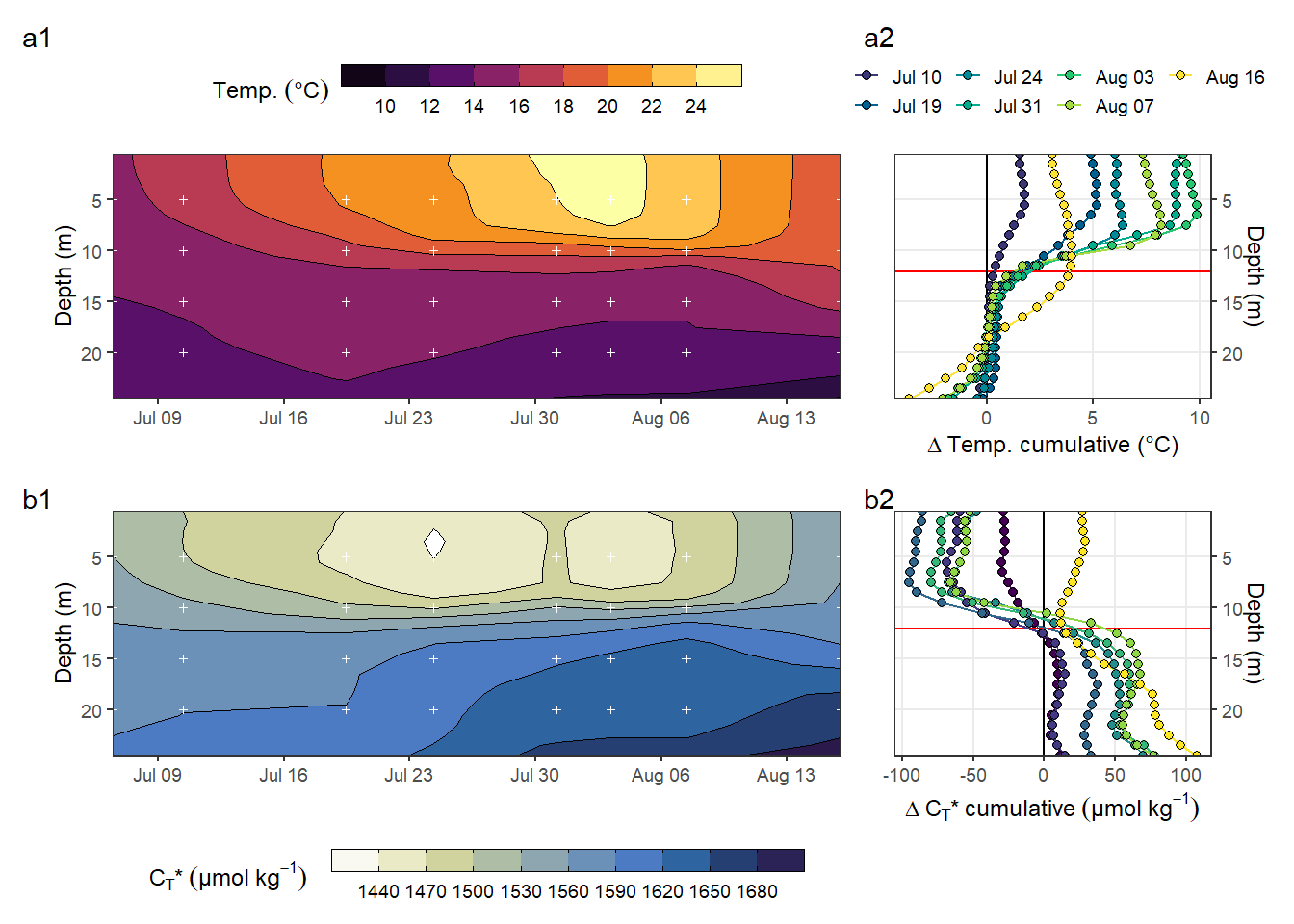
Hovmoeller plots of absolute changes in CT and temperature, combined with profile plots of cumulative changes.
ggsave(
  here::here(
    "output/Plots/Figures_publication/article",
    "Fig_4.pdf"
  ),
  width = 175,
  height = 150,
  dpi = 300,
  units = "mm"
)

ggsave(
  here::here(
    "output/Plots/Figures_publication/article",
    "Fig_4.png"
  ),
  width = 175,
  height = 140,
  dpi = 300,
  units = "mm"
)

rm(p_CT_star_hov, bin_CT_star, p_tem_hov, bin_Tem, p_CT_star_ID_cum, p_tem_ID_cum,
   cum_cruise_dates, viridis_cum_cruise_dates, grid_raster)
8.2 Incremental changes
bin_CT_star <- 2.5

CT_star_hov <- tm_profiles_ID_long %>%
  filter(var == "CT_star") %>%
  ggplot() +
  geom_contour_fill(
    aes(x = date_time_ID_ref, y = dep, z = value_diff_daily),
    breaks = MakeBreaks(bin_CT_star),
    col = "black"
  ) +
  geom_point(
    aes(x = date_time_ID, y = c(24.5)),
    size = 3, shape = 24, fill = "white"
  ) +
  scale_fill_divergent(breaks = MakeBreaks(bin_CT_star),
                       guide = "colorstrip",
                       name = "CT_star") +
  scale_y_reverse() +
  scale_x_datetime(breaks = "week", date_labels = "%d %b") +
  coord_cartesian(expand = 0) +
  theme(axis.title.x = element_blank(),
        axis.text.x = element_blank())

bin_Tem <- 0.1

Tem_hov <- tm_profiles_ID_long %>%
  filter(var == "tem") %>%
  ggplot() +
  geom_contour_fill(
    aes(x = date_time_ID_ref, y = dep, z = value_diff_daily),
    breaks = MakeBreaks(bin_Tem),
    col = "black"
  ) +
  geom_point(
    aes(x = date_time_ID, y = c(24.5)),
    size = 3, shape = 24, fill = "white"
  ) +
  scale_fill_divergent(breaks = MakeBreaks(bin_Tem),
                       guide = "colorstrip",
                       name = "tem") +
  scale_y_reverse() +
  scale_x_datetime(breaks = "week", date_labels = "%d %b") +
  coord_cartesian(expand = 0) +
  theme(axis.title.x = element_blank())

CT_star_hov / Tem_hov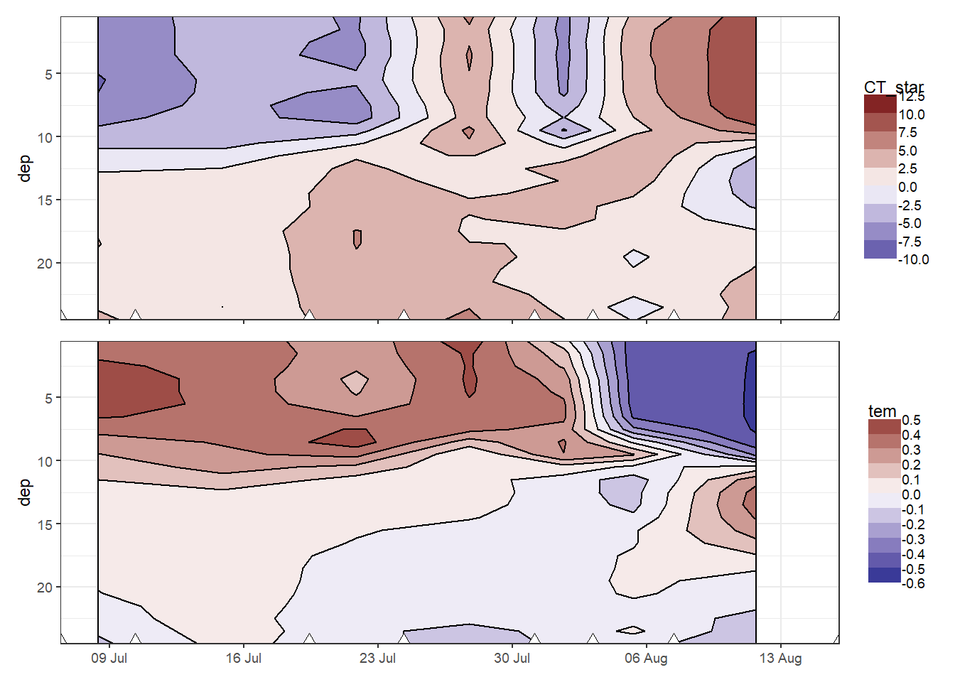
Hovmoeller plots of daily changes in CT and temperature. Note that calculated value of change (in contrast to absolute and cumulative values) are referred to the mean dates inbetween cruise, and are not extrapolated to the full observational period.
rm(CT_star_hov, bin_CT_star, Tem_hov, bin_Tem)8.3 Cumulative changes
bin_CT_star <- 20

CT_star_hov <- tm_profiles_ID_long %>%
  filter(var == "CT_star") %>%
  ggplot() +
  geom_contour_fill(
    aes(x = date_time_ID, y = dep, z = value_cum),
    breaks = MakeBreaks(bin_CT_star),
    col = "black"
  ) +
  geom_point(
    aes(x = date_time_ID, y = c(24.5)),
    size = 3,
    shape = 24,
    fill = "white"
  ) +
  scale_fill_divergent(breaks = MakeBreaks(bin_CT_star),
                       guide = "colorstrip",
                       name = "CT_star") +
  scale_y_reverse() +
  scale_x_datetime(breaks = "week", date_labels = "%d %b") +
  coord_cartesian(expand = 0) +
  theme(axis.title.x = element_blank(),
        axis.text.x = element_blank())

bin_Tem <- 2

Tem_hov <- tm_profiles_ID_long %>%
  filter(var == "tem") %>%
  ggplot() +
  geom_contour_fill(
    aes(x = date_time_ID, y = dep, z = value_cum),
    breaks = MakeBreaks(bin_Tem),
    col = "black"
  ) +
  geom_point(
    aes(x = date_time_ID, y = c(24.5)),
    size = 3,
    shape = 24,
    fill = "white"
  ) +
  scale_fill_divergent(breaks = MakeBreaks(bin_Tem),
                       guide = "colorstrip",
                       name = "tem") +
  scale_y_reverse() +
  scale_x_datetime(breaks = "week", date_labels = "%d %b") +
  coord_cartesian(expand = 0) +
  theme(axis.title.x = element_blank())

CT_star_hov / Tem_hov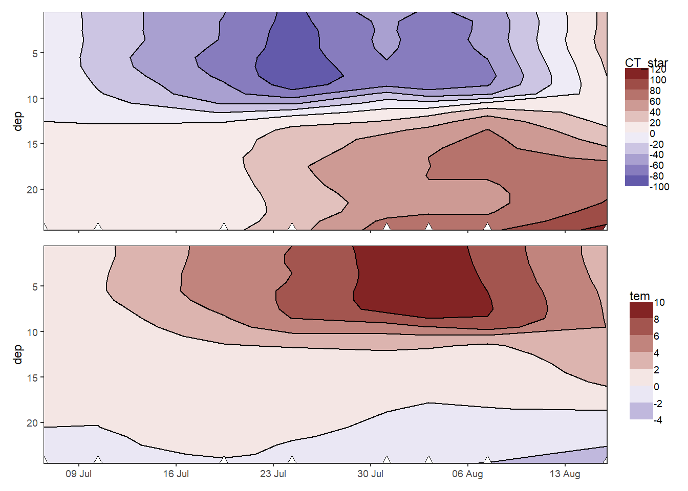
Hovmoeller plotm of cumulative changes in CT and temperature.
rm(CT_star_hov, bin_CT_star, Tem_hov, bin_Tem)9 Depth-integration of CT*
A critical first step for the determination of net community production (NCP) is the integration of observed changes in CT* over depth. Two approaches were tested:
- Integration of changes in CT* over a predefined, fixed water depth
- Integration of changes in CT* over a mixed layer depth (MLD)
Both approaches deliver depth-integrated, incremental changes of CT* ( iCT* ) between cruise dates. Those were summed up to derive a trajectory of cumulative integrated CT* changes.
9.1 Fixed depths approach
Incremental and cumulative CT* changes between cruise dates were integrated across the water columns down to predefined depth limits. This was done separately for observed positive/negative changes in CT*, as well as for the total observed changes.
Predefined integration depth levels in meters are: 9, 10, 11, 12, 13
9.1.1 Calculate iCT*
# create time series grid data frames
iCT_star_grid_sign <- tm_profiles_ID_long %>%
  select(ID, date_time_ID, date_time_ID_ref) %>%
  unique() %>%
  expand_grid(sign = c("pos", "neg"))

iCT_star_grid_total <- tm_profiles_ID_long %>%
  select(ID, date_time_ID, date_time_ID_ref) %>%
  unique() %>%
  expand_grid(sign = c("total"))

# calculate integrated CT* time series for each fixed integration depth
for (i_dep in parameters$fixed_integration_depths) {

  # calculations for pos/neg changes separately

  # integrate (ie sum up) across depth
  iCT_star_sign_temp <- tm_profiles_ID_long %>%
    filter(var == "CT_star", dep < i_dep) %>%
    mutate(sign = if_else(ID == "180705" &
                            dep == 0.5, "neg", sign)) %>%
    group_by(ID, date_time_ID, date_time_ID_ref, sign) %>%
    summarise(CT_star_i_diff = sum(value_diff) / 1000) %>%
    ungroup()

  # calculate cumulative values
  iCT_star_sign_temp <- iCT_star_sign_temp %>%
    group_by(sign) %>%
    arrange(date_time_ID) %>%
    mutate(CT_star_i_cum = cumsum(CT_star_i_diff)) %>%
    ungroup()

  # fill empty values
  iCT_star_sign_temp <-
    full_join(iCT_star_sign_temp, iCT_star_grid_sign) %>%
    arrange(sign, date_time_ID) %>%
    fill(CT_star_i_cum)

  # calculations for total changes

  # integrate (ie sum up) across depth
  iCT_star_total_temp <- tm_profiles_ID_long %>%
    filter(var == "CT_star", dep < i_dep) %>%
    group_by(ID, date_time_ID, date_time_ID_ref) %>%
    summarise(CT_star_i_diff = sum(value_diff) / 1000) %>%
    ungroup()

  # calculate cumulative values
  iCT_star_total_temp <- iCT_star_total_temp %>%
    arrange(date_time_ID) %>%
    mutate(CT_star_i_cum = cumsum(CT_star_i_diff)) %>%
    ungroup() %>%
    mutate(sign = "total")

  # fill empty values
  iCT_star_total_temp <-
    full_join(iCT_star_total_temp, iCT_star_grid_total) %>%
    arrange(sign, date_time_ID) %>%
    fill(CT_star_i_cum)


  # join data frames
  iCT_star_temp <-
    bind_rows(iCT_star_sign_temp, iCT_star_total_temp) %>%
    mutate(i_dep = i_dep)

  # bind data for various integration depths
  if (exists("iCT_star")) {
    iCT_star <- bind_rows(iCT_star, iCT_star_temp)
  } else {
    iCT_star <- iCT_star_temp
  }

  rm(iCT_star_temp, iCT_star_sign_temp, iCT_star_total_temp)

}

rm(iCT_star_grid_sign, iCT_star_grid_total)

iCT_star <- iCT_star %>%
  mutate(i_dep = as.factor(i_dep))

iCT_star_fixed_dep <- iCT_star
rm(iCT_star, i_dep)
9.1.2 Time series
As the bulk changes of CT* occur in the surface water, the choice of the exact fixed integration depth has only minor impact on the derived depth integrated time series.
iCT_star_fixed_dep %>%
  ggplot() +
  geom_point(data = cruise_dates, aes(date_time_ID, 0), shape = 21) +
  geom_col(
    aes(date_time_ID_ref, CT_star_i_diff, fill = i_dep),
    position = "dodge",
    alpha = 0.3
  ) +
  geom_line(aes(date_time_ID, CT_star_i_cum, col = i_dep)) +
  scale_color_viridis_d() +
  scale_fill_viridis_d() +
  scale_x_datetime(breaks = "week", date_labels = "%d %b") +
  facet_grid(sign ~ ., scales = "free_y", space = "free_y") +
  theme_bw()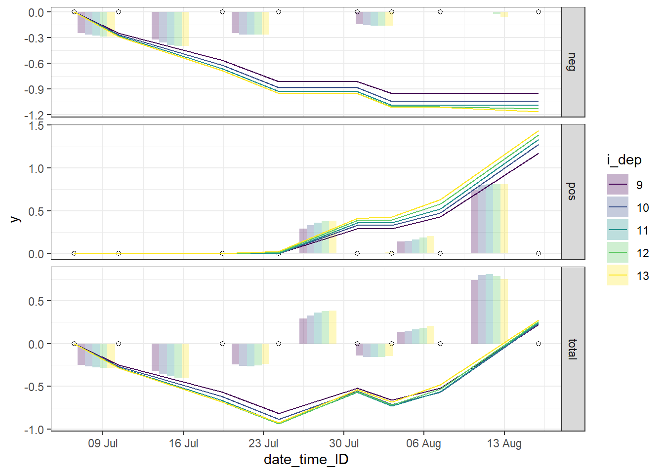
9.2 MLD approach
As an alternative to fixed depth levels, vertical integration as low as the mixed layer depth was tested.
9.2.1 Density calculation
Seawater density Rho was determined from S, T, and p according to TEOS-10.
tm_profiles <- tm_profiles %>%
  mutate(rho = swSigma(
    salinity = sal,
    temperature = tem,
    pressure = dep / 10
  ))
9.2.2 Hydrographical profiles
# hydrographical profiles cruise mean
tm_profiles_ID_mean_hydro <- tm_profiles %>%
  select(-c(station, lat, lon, pCO2_corr, pCO2, CT_star, date_time)) %>%
  group_by(ID, date_time_ID, date_ID, dep) %>%
  summarise_all(list(mean), na.rm = TRUE) %>%
  ungroup()

# hydrographical profiles cruise SD
tm_profiles_ID_sd_hydro <- tm_profiles %>%
  select(-c(station, lat, lon, pCO2_corr, pCO2, CT_star, date_time)) %>%
  group_by(ID, date_time_ID, date_ID, dep) %>%
  summarise_all(list(sd), na.rm = TRUE) %>%
  ungroup()

# convert to long format
tm_profiles_ID_sd_hydro_long <- tm_profiles_ID_sd_hydro %>%
  pivot_longer(sal:rho, names_to = "var", values_to = "sd")

# convert to long format
tm_profiles_ID_mean_hydro_long <- tm_profiles_ID_mean_hydro %>%
  pivot_longer(sal:rho, names_to = "var", values_to = "value")

# join data frames
tm_profiles_ID_hydro_long <-
  inner_join(tm_profiles_ID_mean_hydro_long,
             tm_profiles_ID_sd_hydro_long)

tm_profiles_ID_hydro <- tm_profiles_ID_mean_hydro

rm(
  tm_profiles_ID_mean_hydro_long,
  tm_profiles_ID_mean_hydro,
  tm_profiles_ID_sd_hydro_long,
  tm_profiles_ID_sd_hydro
)
tm_profiles_ID_hydro_long %>%
ggplot(aes(value, dep, col = ID)) +
geom_point() +
geom_path() +
scale_y_reverse() +
scale_color_viridis_d() +
facet_wrap( ~ var, scales = "free_x")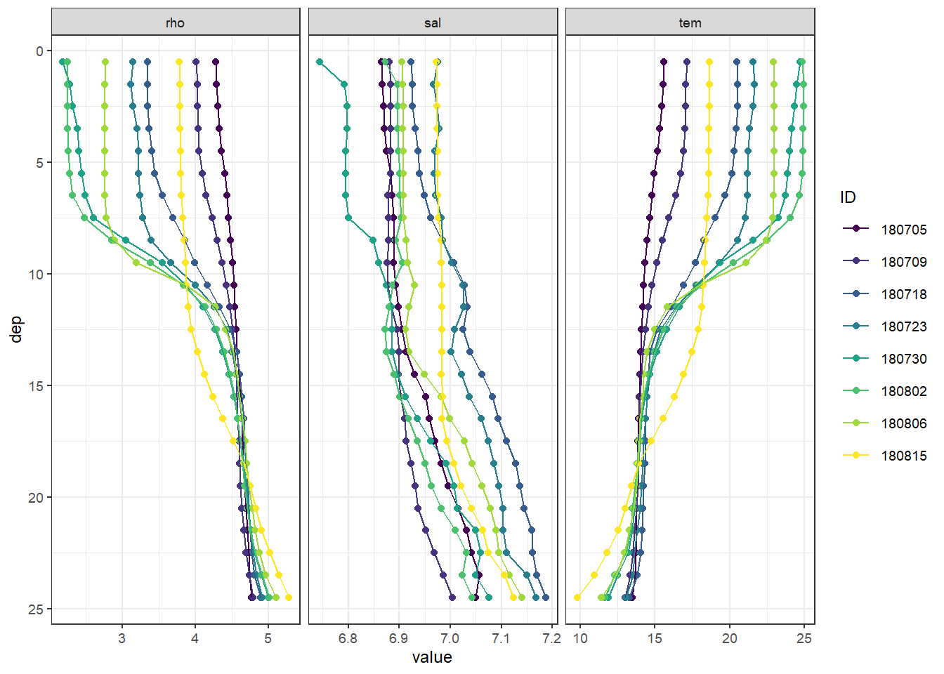
Mean vertical profiles per cruise day across all stations.
9.2.3 MLD calculation
Mixed layer depth (MLD) was determined based on the difference between density at the surface and at depth, for a range of density criteria: 0.1, 0.2, 0.5
tm_profiles_ID_hydro <-
  expand_grid(tm_profiles_ID_hydro,
              rho_lim = parameters$rho_lim_integration_depths)

# calculate MLD for each rho threshold
MLD <- tm_profiles_ID_hydro  %>%
  arrange(dep) %>%
  group_by(ID, date_time_ID, rho_lim) %>%
  mutate(d_rho = rho - first(rho)) %>%
  filter(d_rho > rho_lim) %>%
  summarise(MLD = min(dep)) %>%
  ungroup()
9.2.4 Daily density profiles
tm_profiles_ID_hydro <-
  full_join(tm_profiles_ID_hydro, MLD) %>%
  mutate(rho_lim = as.factor(rho_lim))

tm_profiles_ID_hydro %>%
  arrange(dep) %>%
  ggplot(aes(rho, dep)) +
  geom_hline(aes(yintercept = MLD, col = rho_lim)) +
  geom_path() +
  scale_y_reverse() +
  scale_color_brewer(palette = "Set1") +
  facet_wrap( ~ ID) +
  theme_bw()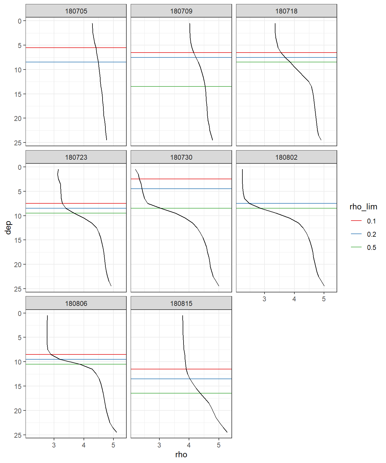
Mean density profiles and MLD per cruise dates (ID).
9.2.5 MLD timeseries
MLD <- MLD %>%
  mutate(rho_lim = as.factor(rho_lim))

MLD %>%
  ggplot(aes(date_time_ID, MLD, col = rho_lim)) +
  geom_hline(yintercept = 0) +
  geom_point() +
  geom_path() +
  scale_color_brewer(palette = "Set1") +
  scale_y_reverse() +
  scale_x_datetime(breaks = "week", date_labels = "%d %b") +
  labs(x = "")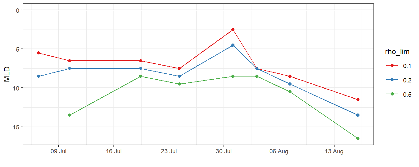
9.2.6 Calculate iCT*
iCT_star <- tm_profiles_ID_long %>%
  filter(var == "CT_star")

# join CT and MLD data frame
iCT_star <- full_join(iCT_star, MLD)

# filter data at depth below MLD
iCT_star <- iCT_star %>%
  filter(dep <= MLD)

# calculate incremental changes
iCT_star <- iCT_star %>%
  group_by(ID, date_time_ID, date_time_ID_ref, rho_lim) %>%
  summarise(CT_star_i_diff = sum(value_diff)/1000) %>%
  ungroup()

# calculate cumulative changes
iCT_star <- iCT_star %>%
  group_by(rho_lim) %>%
  arrange(date_time_ID) %>%
  mutate(CT_star_i_cum = cumsum(CT_star_i_diff)) %>%
  ungroup()

iCT_star_MLD <- iCT_star

rm(iCT_star, MLD, tm_profiles_ID_hydro, tm_profiles_ID_hydro_long)
9.2.7 Time series
iCT_star_MLD %>%
  ggplot() +
  geom_point(data = cruise_dates, aes(date_time_ID, 0), shape = 21) +
  geom_col(
    aes(date_time_ID_ref, CT_star_i_diff, fill = rho_lim),
    position = "dodge",
    alpha = 0.3
  ) +
  geom_line(aes(date_time_ID, CT_star_i_cum, col = rho_lim)) +
  scale_color_viridis_d() +
  scale_fill_viridis_d() +
  scale_x_datetime(breaks = "week", date_labels = "%d %b") +
  theme_bw()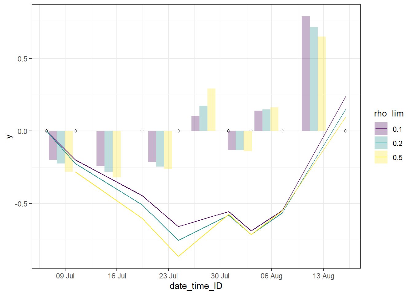
9.3 Comparison of approaches
In the following, all cumulative iCT* trajectories are displayed. Highlighted are those obtained for the fixed depth approach with 12 m limit, and the MLD approach with a standard density threshold of 0.1 kg/m3.
# join data frames with MLD and fixed integration depth
iCT_star <- full_join(iCT_star_fixed_dep, iCT_star_MLD)

# change column types
iCT_star <- iCT_star %>%
  mutate(group = paste(
    as.character(sign),
    as.character(i_dep),
    as.character(rho_lim)
  ))

iCT_star %>%
  arrange(date_time_ID) %>%
  ggplot() +
  geom_hline(yintercept = 0) +
  geom_line(aes(date_time_ID, CT_star_i_cum,
                group = group), col = "grey") +
  geom_line(
    data = iCT_star_fixed_dep %>% filter(i_dep == parameters$i_dep_lim, sign == "total"),
    aes(date_time_ID, CT_star_i_cum, col = "12m - total")
  ) +
  geom_line(data = iCT_star_MLD %>% filter(rho_lim == parameters$rho_lim),
            aes(date_time_ID, CT_star_i_cum, col = "MLD - 0.1")) +
  scale_color_brewer(palette = "Set1", name = "Integration depth") +
  geom_point(data = cruise_dates, aes(date_time_ID, 0), shape = 21) +
  scale_x_datetime(breaks = "week", date_labels = "%d %b")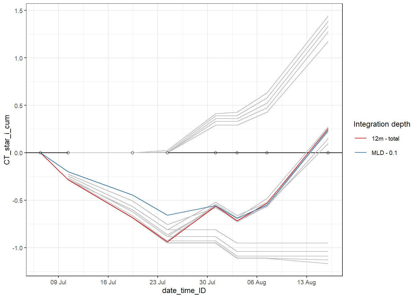
rm(iCT_star, iCT_star_MLD)10 Best–guess NCP estimate
In order to derive an estimate of the net community production NCP (which is equivalent to the formed organic matter that can be exported from the investigated surface layer), two steps are required:
decision about the most appropriate iCT trajectory
correction of quantifiable CO2 fluxes in and out of the investigated water volume during the period of interest, this includes:
- Air-sea CO2 fluxes
- CO2 fluxes due to vertical mixing
- CO2 fluxes due to lateral transport of water masses (not corrected here)
10.1 Best iCT* estimate
To determine the optimum depth for the CT* integration we investigated the vertical distribution of cumulative temperature and CT* changes on the peak of the productivity signal on June 23:
# subset data from bloom peak
tm_profiles_ID_long_180723 <- tm_profiles_ID_long %>%
  filter(ID == 180723,
         var == "CT_star")

p_tm_profiles_ID_long <- tm_profiles_ID_long_180723 %>%
  arrange(dep) %>%
  ggplot(aes(value_cum, dep)) +
  geom_vline(xintercept = 0) +
  geom_hline(yintercept = 12, col = "red") +
  geom_point() +
  geom_path() +
  scale_y_reverse() +
  labs(x = "Cumulative change of CT_star on July 23 (180723)") +
  theme(legend.position = "left")

# calculate column integral
tm_profiles_ID_long_180723_dep <- tm_profiles_ID_long_180723 %>%
  select(dep, value_cum) %>%
  filter(value_cum < 0) %>%
  arrange(dep) %>%
  mutate(
    value_cum_i = sum(value_cum),
    value_cum_dep = cumsum(value_cum),
    value_cum_i_rel = value_cum_dep / value_cum_i * 100
  )

p_tm_profiles_ID_long_rel <- tm_profiles_ID_long_180723_dep %>%
  ggplot(aes(value_cum_i_rel, dep)) +
  geom_hline(yintercept = 12, col = "red") +
  geom_vline(xintercept = 90) +
  geom_point() +
  geom_line() +
  scale_y_reverse(limits = c(25, 0)) +
  scale_x_continuous(breaks = seq(0, 100, 10)) +
  labs(y = "Depth (m)", x = "Relative contribution on July 23") +
  theme_bw()

p_tm_profiles_ID_long + p_tm_profiles_ID_long_rel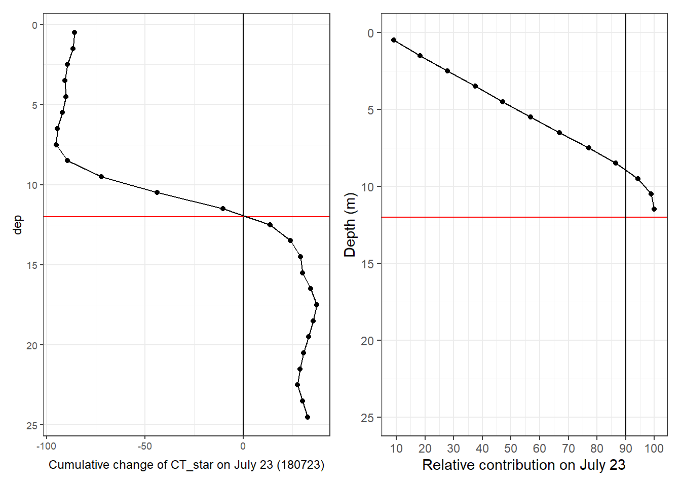
rm(
  tm_profiles_ID_long_180723,
  tm_profiles_ID_long_180723_dep,
  p_tm_profiles_ID_long,
  p_tm_profiles_ID_long_rel
)
# subset data from bloom peak
tm_profiles_ID_long_180723 <- tm_profiles_ID_long %>%
filter(ID == 180723,
var == "tem")
p_tm_profiles_ID_long <- tm_profiles_ID_long_180723 %>%
arrange(dep) %>%
ggplot(aes(value_cum, dep)) +
geom_vline(xintercept = 0) +
geom_hline(yintercept = 12, col = "red") +
geom_point() +
geom_path() +
scale_y_reverse() +
labs(x = "Cumulative change of Temp on July 23") +
theme(legend.position = "left")
# calculate column integral
tm_profiles_ID_long_180723_dep <- tm_profiles_ID_long_180723 %>%
select(dep, value_cum) %>%
filter(value_cum > 0) %>%
arrange(dep) %>%
mutate(
value_cum_i = sum(value_cum),
value_cum_dep = cumsum(value_cum),
value_cum_i_rel = value_cum_dep / value_cum_i * 100
)
p_tm_profiles_ID_long_rel <- tm_profiles_ID_long_180723_dep %>%
ggplot(aes(value_cum_i_rel, dep)) +
geom_hline(yintercept = 12, col = "red") +
geom_vline(xintercept = 90) +
geom_point() +
geom_line() +
scale_y_reverse(limits = c(25, 0)) +
scale_x_continuous(breaks = seq(0, 100, 10)) +
labs(y = "Depth (m)", x = "Relative contribution on July 23") +
theme_bw()
p_tm_profiles_ID_long + p_tm_profiles_ID_long_rel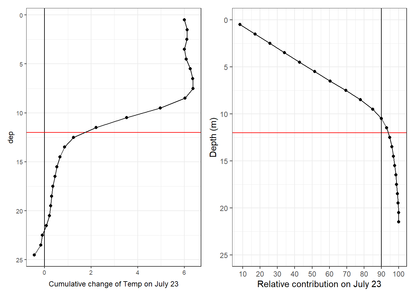
rm(
  tm_profiles_ID_long_180723,
  tm_profiles_ID_long_180723_dep,
  p_tm_profiles_ID_long,
  p_tm_profiles_ID_long_rel
)
The cummulative iCT* trajectory determined by integration of CT* to a fixed water depth of 12 m was used for NCP calculation for the following reasons:
During the first productivity pulse that lasted until July 23:
- no negative CT* changes were detected below that depth
- cumulative CT* switch sign at that depth
- 95% of the cumulative warming signal appears across that depth
MLD were too shallow to cover all observed negative CT* changes
# extract CT data for fixed depth approach, depth limit 10m
NCP <- iCT_star_fixed_dep %>%
  filter(i_dep == parameters$i_dep_lim, sign == "total") %>%
  select(-c(sign, i_dep))

rm(iCT_star_fixed_dep)

NCP <- NCP %>%
  select(ID, date_time = date_time_ID, date_time_ID_ref, CT_star_i_diff, CT_star_i_cum)

# date of the second last cruise
date_180806 <- unique(NCP$date_time)[7]
10.2 Air-Sea CO2 flux
10.2.1 Surface water time series
The mean pCO2 of each cruise recorded in profiling-mode (stations only) and depths < 6`m was used for gas exchange calculations.
# surface time series data in long format
tm_profiles_surface_long <- tm_profiles %>%
  filter(dep < parameters$surface_dep) %>%
  select(date_time = date_time_ID, ID, tem, pCO2 = pCO2, CT_star) %>%
  pivot_longer(tem:CT_star, values_to = "value", names_to = "var")

tm_profiles_surface_long_ID <- tm_profiles_surface_long %>%
  group_by(ID, date_time, var) %>%
  summarise_all(list( ~ mean(.), ~ sd(.), ~ min(.), ~ max(.))) %>%
  ungroup()

rm(tm_profiles_surface_long)


# plot surface time series
p_pCO2_surf <- tm_profiles_surface_long_ID %>%
  filter(var == "pCO2") %>%
  ggplot(aes(x = date_time)) +
  geom_vline(data = cruise_dates, aes(xintercept = date_time_ID), col = "grey92") +
  geom_ribbon(aes(
    ymin = mean - sd,
    ymax = mean + sd,
    fill = "\u00B1 SD"
  ), alpha = 0.2) +
  geom_path(aes(y = mean)) +
  geom_point(aes(y = mean)) +
  scale_color_manual(name = "",
                     values = "black",
                     guide = FALSE) +
  scale_fill_manual(name = "",
                    values = "black",
                    guide = FALSE) +
  scale_x_datetime(date_breaks = "week") +
  labs(y = expression(atop(italic(p) * CO[2], (mu * atm)))) +
  theme(
    axis.title.x = element_blank(),
    axis.text.x = element_blank(),
    axis.ticks.x = element_blank(),
    legend.title = element_blank(),
    plot.margin = margin(0, 0, 0, 0, "cm"),
    panel.grid.minor = element_blank(),
    panel.grid.major.x = element_blank()
  )

p_tem_surf <- tm_profiles_surface_long_ID %>%
  filter(var == "tem") %>%
  ggplot(aes(x = date_time)) +
  geom_vline(data = cruise_dates, aes(xintercept = date_time_ID), col = "grey92") +
  geom_ribbon(aes(
    ymin = mean - sd,
    ymax = mean + sd,
    fill = "Mean \u00B1 SD"
  ),
  alpha = 0.2) +
  geom_path(aes(y = mean, col = "Mean \u00B1 SD")) +
  geom_point(aes(y = mean, col = "Mean \u00B1 SD")) +
  scale_color_manual(name = "Sensor data", values = "black") +
  scale_fill_manual(name = "Sensor data", values = "black") +
  scale_x_datetime(date_breaks = "week") +
  labs(y = expression(atop("SST", "(\u00B0C)"))) +
  theme(
    axis.title.x = element_blank(),
    axis.text.x = element_blank(),
    axis.ticks.x = element_blank(),
    legend.key.height = unit(5, "mm"),
    legend.key.width = unit(5,"mm"),
    plot.margin = margin(0, 0, 0, 0, "cm"),
    panel.grid.minor = element_blank(),
    panel.grid.major.x = element_blank()
  )


p_CT_star_surf <-
  tm_profiles_surface_long_ID %>%
  filter(var == "CT_star") %>%
  ggplot() +
  geom_vline(data = cruise_dates, aes(xintercept = date_time_ID), col = "grey92") +
  geom_ribbon(aes(
    x = date_time,
    ymin = mean - sd,
    ymax = mean + sd,
    fill = "\u00B1 SD"
  ),
  alpha = 0.2) +
  geom_path(aes(x = date_time, y = mean)) +
  geom_point(aes(x = date_time, y = mean)) +
  scale_color_manual(name = "", values = "black", guide = FALSE) +
  scale_fill_manual(name = "", values = "black", guide = FALSE) +
  new_scale_color() +
  geom_linerange(
    data = tb_surface_station_mean %>%
      filter(var == "CT_star"),
    aes(
      x = date_time_ID,
      ymin = value_mean - value_sd,
      ymax = value_mean + value_sd,
      color = "Mean \u00B1 SD"
    )
  ) +
  geom_point(
    data = tb_surface_station_mean %>%
      filter(var == "CT_star"),
    aes(x = date_time_ID,
        y = value_mean,
        color = "Mean \u00B1 SD")
  ) +
  scale_color_manual(name = "Bottle data", values = "red") +
  scale_x_datetime(date_breaks = "week") +
  labs(y = expression(atop(paste(C[T], "*"),
                           (mu * mol ~ kg ^ {
                             -1
                           })))) +
  theme(
    axis.title.x = element_blank(),
    axis.text.x = element_blank(),
    axis.ticks.x = element_blank(),
    legend.key.height = unit(5, "mm"),
    legend.key.width = unit(5,"mm"),
    plot.margin = margin(0, 0, 0, 0, "cm"),
    panel.grid.minor = element_blank(),
    panel.grid.major.x = element_blank()
  )


p_pCO2_surf + p_tem_surf + p_CT_star_surf +
  plot_layout(ncol = 1)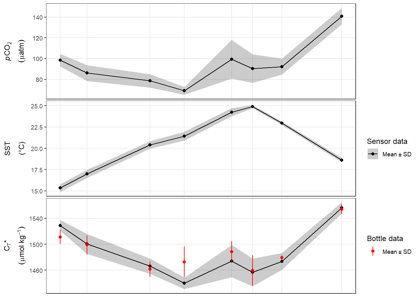
start <- min(tm_profiles_surface_long_ID$date_time)
end   <- max(tm_profiles_surface_long_ID$date_time)
10.2.2 Surface water table
The mean values per cruise and regional variability of surface water parameters was:
tm_profiles_surface_long_ID %>%
  arrange(var) %>%
  kable() %>%
  add_header_above() %>%
  kable_styling(full_width = FALSE) %>%
scroll_box(height = "400px")| ID | date_time | var | mean | sd | min | max |
|---|---|---|---|---|---|---|
| 180705 | 2018-07-06 11:14:37 | CT_star | 1529.05101 | 8.2883766 | 1511.47632 | 1542.59218 |
| 180709 | 2018-07-10 08:45:38 | CT_star | 1500.58938 | 15.3560456 | 1471.05824 | 1520.34626 |
| 180718 | 2018-07-19 10:01:48 | CT_star | 1466.23938 | 11.6934378 | 1447.28428 | 1498.63509 |
| 180723 | 2018-07-24 07:58:29 | CT_star | 1439.95418 | 8.8650660 | 1415.45950 | 1455.43971 |
| 180730 | 2018-07-31 03:45:31 | CT_star | 1474.15099 | 25.0365019 | 1440.83302 | 1519.20433 |
| 180802 | 2018-08-03 04:13:45 | CT_star | 1456.68067 | 21.4027858 | 1431.16303 | 1508.09978 |
| 180806 | 2018-08-07 09:28:50 | CT_star | 1473.58590 | 13.0806501 | 1447.00955 | 1491.52912 |
| 180815 | 2018-08-16 00:08:48 | CT_star | 1556.16806 | 8.4373691 | 1540.84549 | 1570.11761 |
| 180705 | 2018-07-06 11:14:37 | pCO2 | 98.47996 | 6.0910301 | 87.19089 | 110.24034 |
| 180709 | 2018-07-10 08:45:38 | pCO2 | 86.07135 | 7.6184441 | 72.44729 | 96.88215 |
| 180718 | 2018-07-19 10:01:48 | pCO2 | 78.60290 | 6.4959027 | 69.81329 | 101.52258 |
| 180723 | 2018-07-24 07:58:29 | pCO2 | 68.93034 | 3.6813844 | 59.87285 | 75.31610 |
| 180730 | 2018-07-31 03:45:31 | pCO2 | 99.46161 | 18.7131469 | 79.74148 | 134.65088 |
| 180802 | 2018-08-03 04:13:45 | pCO2 | 90.30475 | 13.7987160 | 76.75694 | 126.69686 |
| 180806 | 2018-08-07 09:28:50 | pCO2 | 92.32443 | 7.6007064 | 78.38499 | 103.82754 |
| 180815 | 2018-08-16 00:08:48 | pCO2 | 140.90864 | 7.9648078 | 126.49526 | 154.87771 |
| 180705 | 2018-07-06 11:14:37 | tem | 15.33978 | 0.4458508 | 14.56363 | 16.25533 |
| 180709 | 2018-07-10 08:45:38 | tem | 16.98802 | 0.4766441 | 16.06309 | 17.89843 |
| 180718 | 2018-07-19 10:01:48 | tem | 20.39976 | 0.4285885 | 19.76884 | 21.24747 |
| 180723 | 2018-07-24 07:58:29 | tem | 21.42724 | 0.5108960 | 21.00930 | 22.93845 |
| 180730 | 2018-07-31 03:45:31 | tem | 24.24527 | 0.4602385 | 23.64305 | 25.31519 |
| 180802 | 2018-08-03 04:13:45 | tem | 24.88713 | 0.1846099 | 24.53541 | 25.27263 |
| 180806 | 2018-08-07 09:28:50 | tem | 22.95573 | 0.2038156 | 22.60425 | 23.35020 |
| 180815 | 2018-08-16 00:08:48 | tem | 18.62651 | 0.2752079 | 18.13858 | 19.01634 |
10.2.3 Surface water variability
For the time period of the production pulse from July 6 - 24, the regional variability within the study area can be summarized as:
tm_profiles_surface_long_ID %>%
  filter(date_time < ymd("2018-07-26")) %>%
  group_by(var) %>%
  summarise(SD_mean = mean(sd)) %>%
  ungroup() %>%
  kable() %>%
  add_header_above() %>%
kable_styling(full_width = FALSE)| var | SD_mean |
|---|---|
| CT_star | 11.0507315 |
| pCO2 | 5.9716903 |
| tem | 0.4654949 |
10.2.4 Wind and atm. pCO2
Meteorological data were recorded on the flux tower located on Östergarnsholm island.
# read data
og <-
  read_csv(here::here("data/intermediate/_summarized_data_files",
                      "og.csv"))

# filter time period of field study
og <- og %>%
  filter(date_time > start,
         date_time < end)

rm(end, start)
10.2.5 Conversion to U10
Wind speed was determined at 12 and converted to 10 m above sea level, to be used for gas exchange calculation.
og <- og %>%
  mutate(wind = wind.scale.base(wnd = wind, wnd.z = 12))
10.2.6 Time series
p_pCO2_atm <- og %>%
  ggplot(aes(x = date_time)) +
  geom_vline(data = cruise_dates, aes(xintercept = date_time_ID), col = "grey92") +
  geom_path(aes(y = pCO2_atm)) +
  scale_x_datetime(date_breaks = "week") +
  labs(y = expression(atop(italic(p) * CO["2,atm"], (mu * atm)))) +
  theme(
    axis.title.x = element_blank(),
    axis.text.x = element_blank(),
    axis.ticks.x = element_blank(),
    plot.margin = margin(0, 0, 0, 0, "cm"),
    panel.grid.minor = element_blank(),
    panel.grid.major.x = element_blank()
  )

p_wind <- og %>%
  ggplot(aes(x = date_time)) +
  geom_vline(data = cruise_dates, aes(xintercept = date_time_ID), col = "grey92") +
  geom_path(aes(y = wind)) +
  scale_x_datetime(date_breaks = "week") +
  labs(y = expression(atop(U["10"], (m ~ s ^ {
    -1
  })))) +
  theme(
    axis.title.x = element_blank(),
    axis.text.x = element_blank(),
    axis.ticks.x = element_blank(),
    legend.title = element_blank(),
    plot.margin = margin(0, 0, 0, 0, "cm"),
    panel.grid.minor = element_blank(),
    panel.grid.major.x = element_blank()
  )

p_pCO2_atm + p_wind +
  plot_layout(ncol = 1) +
  plot_layout(guides = 'collect')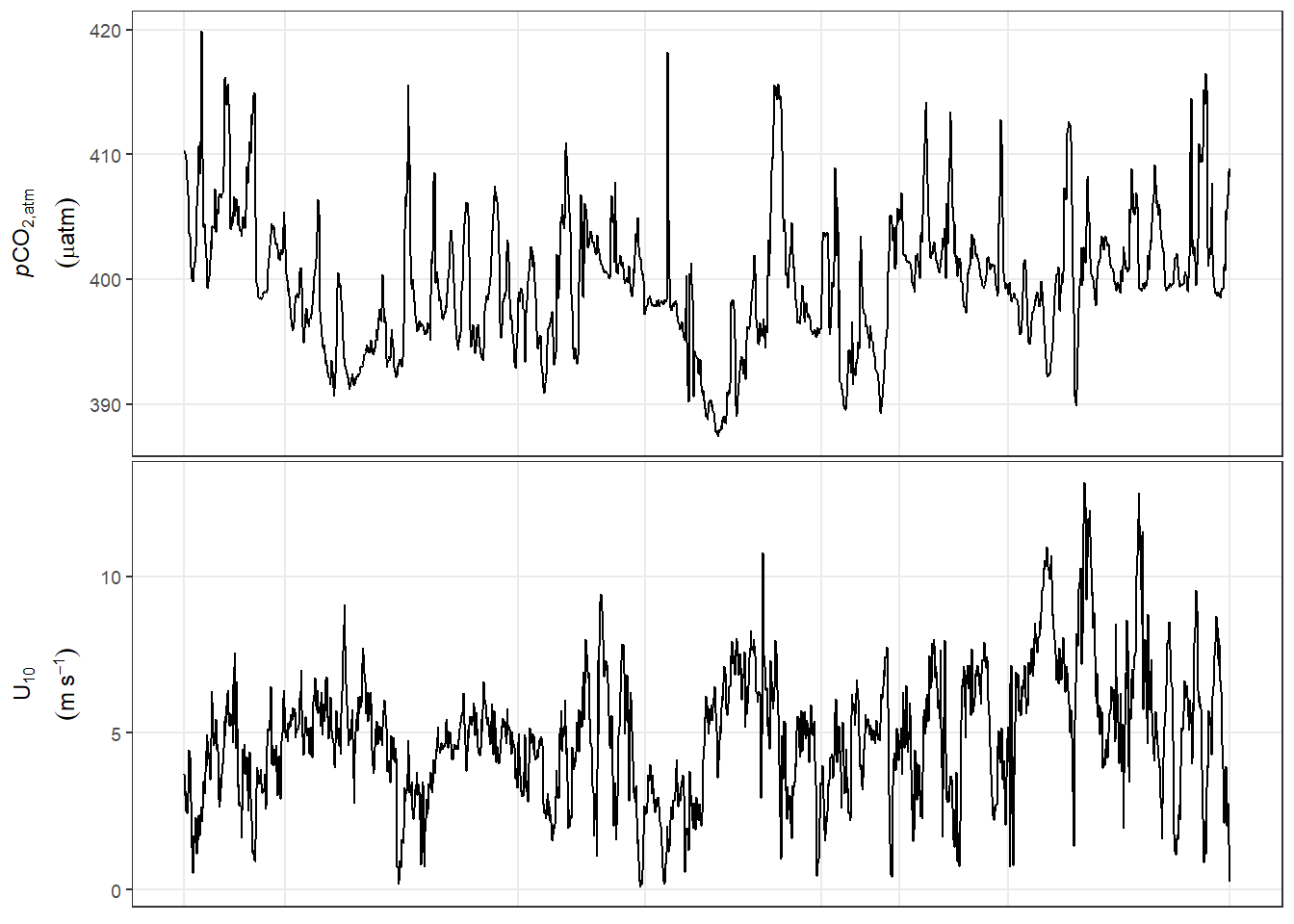
10.2.7 Temporal interpolation
Data sets for atmospheric and seawater observations were merged and seawater date were interpolated to the time stamp of atmospheric data.
tm_profiles_surface_ID <- tm_profiles_surface_long_ID %>%
  filter(var %in% c("pCO2", "tem")) %>%
  select(date_time:mean) %>%
  pivot_wider(names_from = "var", values_from = "mean")

rm(tm_profiles_surface_long_ID)

tm_og <- full_join(og, tm_profiles_surface_ID) %>%
  arrange(date_time)

tm_og <- tm_og %>%
  mutate(
    pCO2 = approxfun(date_time, pCO2)(date_time),
    tem = approxfun(date_time, tem)(date_time),
    wind = approxfun(date_time, wind)(date_time)
  ) %>%
  filter(!is.na(pCO2_atm))

rm(tm_profiles_surface_ID, og)
10.2.8 Air-sea fluxes
F = k * dCO2
with
dCO2 = K0 * dpCO2 and
k = coeff * U^2 * (660/Sc)^0.5
Unitm used here are:
dpCO2: µatm
K0: mol atm-1 kg-1
dCO2: µmol kg-1
wind speed U: m s-1
coeff for k calculation (eg 0.251 in W14): cm hr-1 (m s-1)-2
gas transfer velocities k: cm hr-1 (= 60 x 60 x 100 m s-1)
air sea CO2 flux F: mol m–2 d–1
conversion between the unit of k * dCO2 and F requires a factor of 10-5 * 24
# define gas exchange coefficient according to Wanninkhof 2014
Sc_W14 <- function(tem) {
  2116.8 - 136.25 * tem + 4.7353 * tem ^ 2 - 0.092307 * tem ^ 3 + 0.0007555 * tem ^
    4
}

# Sc_W14(20)

tm_og <- tm_og %>%
  mutate(
    dpCO2 = pCO2 - pCO2_atm,
    dCO2  = dpCO2 * K0(S = 6.92, T = tem),
    # W92 = gas_transfer(t = tem, u10 = wind, species = "CO2",
    #                      method = "Wanninkhof1")* 60^2 * 100,
    #k_SM18 = 0.24 * wind^2 * ((1943-119.6*tem + 3.488*tem^2 - 0.0417*tem^3) / 660)^(-0.5),
    k = 0.251 * wind ^ 2 * (Sc_W14(tem) / 660) ^ (-0.5)
  )

# calculate flux F [mol m–2 d–1]
tm_og <- tm_og %>%
  mutate(flux = k * dCO2 * 1e-5 * 24)

rm(Sc_W14)
p_flux_daily <- tm_og %>%
ggplot(aes(x = date_time)) +
geom_vline(data = cruise_dates, aes(xintercept = date_time_ID), col = "grey92") +
geom_path(aes(y = flux)) +
scale_x_datetime(date_breaks = "week") +
labs(y = expression(atop(F["air-sea, daily"], (mol ~ m ^ {
-2
} ~ d ^ {
-1
})))) +
theme(
axis.title.x = element_blank(),
axis.text.x = element_blank(),
axis.ticks.x = element_blank(),
legend.title = element_blank(),
plot.margin = margin(0, 0, 0, 0, "cm"),
panel.grid.minor = element_blank(),
panel.grid.major.x = element_blank()
)# scale flux data from daily to 30 min (measurement freuquency)$
# calculate cumulative fluc
tm_og <- tm_og %>%
mutate(scale = 24 * 2) %>%
mutate(flux_scale = flux / scale) %>%
arrange(date_time) %>%
mutate(flux_cum = cumsum(flux_scale)) %>%
ungroup()
p_flux_cum <- tm_og %>%
ggplot(aes(x = date_time)) +
geom_vline(data = cruise_dates, aes(xintercept = date_time_ID), col = "grey92") +
geom_path(aes(y = flux_cum)) +
scale_fill_discrete(guide = FALSE) +
scale_x_datetime(date_breaks = "week") +
labs(y = expression(atop(F["air-sea, cum"],
(mol ~ m ^ {
-2
})))) +
theme(
axis.title.x = element_blank(),
axis.text.x = element_blank(),
axis.ticks.x = element_blank(),
plot.margin = margin(0, 0, 0, 0, "cm"),
panel.grid.minor = element_blank(),
panel.grid.major.x = element_blank()
)
p_flux_daily + p_flux_cum +
plot_layout(ncol = 1)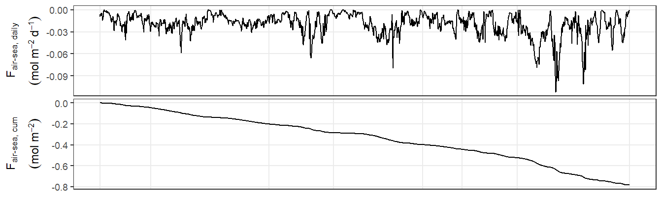
10.2.9 Air-sea flux correction
Correction of iCT* for air-sea CO2 fluxes are based on estimates derived from observation with 30min measurement interval and calculation according to Wanninkhof (2014). The MLD was always shallower 12m, except for the last cruise day. Therefore:
- Cumulative air-sea fluxes can be added completely to iCT* before Aug 7.
- Between Aug 7 and the last cruise on Aug 15 it was assumed, that the CO2 flux was homogeneously mixed down to the deepened thermocline at 17m. The flux correction applied to the upper 12m can therefore be scaled with a factor 12/17.
# calculate cumulative air-sea fluxes affecting surface water column
tm_og_flux <- tm_og %>%
  mutate(
    flux_scale = if_else(
      date_time > date_180806,
      parameters$i_dep_lim / parameters$i_dep_mix_lim * flux_scale,
      flux_scale
    )
  ) %>%
  arrange(date_time) %>%
  mutate(flux_cum = cumsum(flux_scale)) %>%
  select(date_time, flux_cum)


NCP_flux <- full_join(NCP, tm_og_flux) %>%
  arrange(date_time)

rm(tm_og_flux, NCP, tm_og)


# linear interpolation of cumulative changes to frequency of the flux estimates estimates
NCP_flux <- NCP_flux %>%
  mutate(
    CT_star_i_cum = approxfun(date_time, CT_star_i_cum)(date_time),
    flux_cum = approxfun(date_time, flux_cum)(date_time)
  ) %>%
  fill(flux_cum) %>%
  mutate(CT_star_i_flux_cum = CT_star_i_cum + flux_cum)


# calculate cumulative fluxes between cruises
NCP_flux_diff <- NCP_flux %>%
  filter(!is.na(date_time_ID_ref)) %>%
  mutate(flux_diff = flux_cum - lag(flux_cum, default = 0)) %>%
  select(ID, date_time_ID_ref, observed = CT_star_i_diff, flux = flux_diff) %>%
  pivot_longer(cols = "observed":"flux",
               names_to = "var",
               values_to = "value_diff") %>%
  mutate(var = if_else(var == "flux", "air-sea flux", var))
10.3 Vertical mixing
During the last cruise, deeper mixing up to 17m water depth was observed. The entrainment of CT* into the surface layer, was estimated from comparing the actual concentration of CT* in 12-17m before the mixing, to a hypothetical concentration if instantaneous mixing to 17m had happened.
10.3.1 Profiles
The aim is to approximate the CT* entrainment flux between Aug 07 and 16. The relevant profiles are:
viridis_tail <- tail(hcl.colors(nrow(cruise_dates), "viridis"),2)

# calculate mean volume weighted CT* before micing
CT_mix <- tm_profiles_ID_long %>%
  filter(ID == "180806",
         var == "CT_star",
         dep < parameters$i_dep_mix_lim) %>%
  summarise(CT_star_surface = sum(value) / parameters$i_dep_mix_lim) %>%
  pull()

# subset CT* profile before mixing
CT_profile <- tm_profiles_ID_mean %>%
  filter(ID %in% c("180806"))

p_CT_star <- CT_profile %>%
  ggplot() +
  geom_rect(
    data = CT_profile %>% filter(dep > 12, dep < 17),
    aes(
      xmax = CT_star,
      xmin = CT_mix,
      ymax = dep + 0.5,
      ymin = dep - 0.5
    ),
    alpha = 0.2
  ) +
  geom_hline(yintercept = c(12, 17)) +
  geom_segment(aes(
    x = CT_mix,
    xend = CT_mix,
    y = -Inf,
    yend = 17
  ),
  linetype = 2) +
  annotate(
    "text",
    label = as.character(expression(paste(C[T], "*") ~ mix)),
    parse = TRUE,
    x = 1580,
    y = 3,
    size = geom_text_size
  ) +
  annotate(
    "text",
    label = as.character(expression(paste(C[T], "*") ~ flux)),
    parse = TRUE,
    x = 1580,
    y = 14.5,
    size = geom_text_size
  ) +
  geom_path(aes(CT_star, dep, col = ID)) +
  geom_point(aes(CT_star, dep, fill = ID), shape = 21) +
  scale_y_reverse() +
  scale_fill_manual(values = viridis_tail) +
  scale_color_manual(values = viridis_tail) +
  labs(y = "Depth (m)", x = expression(paste(C[T], "*", ~ (µmol ~ kg ^ {
    -1
  })))) +
  theme(
    legend.title = element_blank(),
    axis.text.y = element_blank(),
    axis.ticks.y = element_blank(),
    axis.title.y = element_blank(),
    legend.position = "none",
    panel.grid.minor = element_blank()
  )

# subset temperature profiles before and after mixing
tm_profiles_ID_long_temp <-
  left_join(
    tm_profiles_ID_long %>%
      filter(ID %in% c("180806", "180815"),
             var %in% c("tem")) %>%
      select(-date_ID),
    cruise_dates
  )


p_tem <- tm_profiles_ID_long_temp  %>%
  ggplot() +
  geom_hline(yintercept = c(12, 17)) +
  geom_path(aes(value, dep, col = date_ID)) +
  geom_point(aes(value, dep, fill = date_ID), shape = 21) +
  scale_y_reverse() +
  scale_color_manual(values = viridis_tail, name = "Mean\ncruise date") +
  scale_fill_manual(values = viridis_tail, name = "Mean\ncruise date") +
  labs(y = "Depth (m)", x = expression(paste(Temperature ~ "(\u00B0C)"))) +
  theme(panel.grid.minor = element_blank())

p_tem + p_CT_star +
  plot_layout(guides = 'collect') +
  plot_annotation(tag_levels = 'a')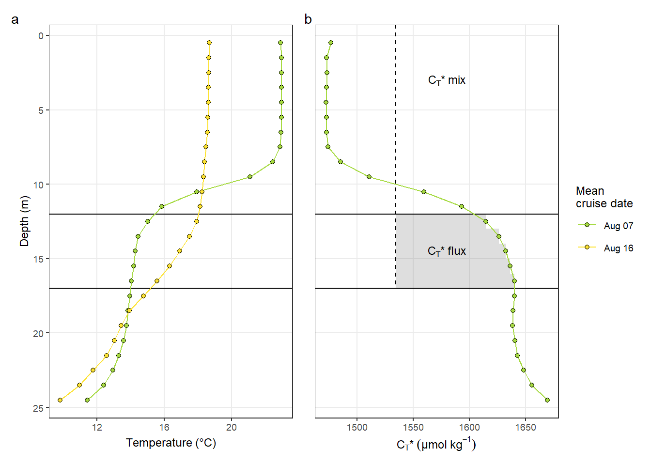
ggsave(
  here::here("output/Plots/Figures_publication/appendix",
             "Fig_C2.pdf"),
  width = 130,
  height = 110,
  dpi = 300,
  units = "mm"
)

ggsave(
  here::here("output/Plots/Figures_publication/appendix",
             "Fig_C2.png"),
  width = 130,
  height = 110,
  dpi = 300,
  units = "mm"
)


rm(p_tem, p_CT_star, CT_profile, tm_profiles_ID_long_temp, viridis_tail)
10.3.2 Mixing correction
The effect of mixing was derived from the integrated difference between CT* and CT* across 12-17m on Aug 07.
# calculate mixing with deep waters
NCP_mix_deep <- tm_profiles_ID_long %>%
  filter(
    ID == "180806",
    var == "CT_star",
    dep < parameters$i_dep_mix_lim,
    dep > parameters$i_dep_lim
  ) %>%
  mutate(CT_star_delta_mix = CT_mix - value) %>%
  summarise(value_diff = sum(CT_star_delta_mix) / 1000) %>%
  mutate(ID = "180815")

NCP_mix_deep_diff <- NCP_mix_deep %>%
  mutate(var = "mixing")

# join flux and mixing correction time series data: incremental
NCP_flux_mix_diff <-
  full_join(NCP_flux_diff, NCP_mix_deep_diff) %>%
  arrange(ID) %>%
  fill(date_time_ID_ref)

NCP_mix_deep <- NCP_mix_deep %>%
  rename(mix_cum = value_diff) %>%
  select(ID, mix_cum)

# join flux and mixing correction time series data: cumulative
NCP_flux_mix <-
  full_join(NCP_flux,
            NCP_mix_deep)

rm(NCP_mix_deep,
   NCP_mix_deep_diff,
   NCP_flux,
   NCP_flux_diff,
   date_180806)

# apply mixing correction
NCP_flux_mix <- NCP_flux_mix %>%
  arrange(date_time) %>%
  fill(ID) %>%
  mutate(
    mix_cum = if_else(ID %in% c("180806", 180815), mix_cum, 0),
    mix_cum = na.approx(mix_cum),
    CT_star_i_flux_mix_cum = CT_star_i_flux_cum + mix_cum
  )
# reorder factors for plotting
NCP_flux_mix_diff <- NCP_flux_mix_diff %>%
mutate(var = factor(var, c("observed", "air-sea flux", "mixing")))
NCP_flux_mix_long <- NCP_flux_mix %>%
select(date_time,
CT_star_i_cum,
CT_star_i_flux_cum,
CT_star_i_flux_mix_cum) %>%
pivot_longer(CT_star_i_cum:CT_star_i_flux_mix_cum,
values_to = "value",
names_to = "var") %>%
mutate(
var = fct_recode(
var,
observed = "CT_star_i_cum",
`air-sea flux corrected` = "CT_star_i_flux_cum",
`air-sea flux + mixing\ncorrected (- NCP)` = "CT_star_i_flux_mix_cum"
)
)
p_iCT_star <- NCP_flux_mix_long %>%
arrange(date_time) %>%
ggplot() +
geom_col(
data = NCP_flux_mix_diff,
aes(date_time_ID_ref, value_diff, fill = var),
position = position_dodge2(preserve = "single"),
alpha = 0.5
) +
geom_vline(data = cruise_dates, aes(xintercept = date_time_ID), col = "grey92") +
geom_point(data = cruise_dates, aes(date_time_ID, 0), shape = 3) +
geom_hline(yintercept = 0) +
geom_line(aes(date_time, value, col = var)) +
scale_x_datetime(date_breaks = "week",
date_labels = "%b %d") +
scale_fill_brewer(palette = "Dark2", name = "Incremental changes") +
scale_color_brewer(palette = "Dark2", name = "Cumulative changes") +
labs(y = expression(atop(Integrated ~ Delta ~ paste(C[T], "*"), (mol ~ m ^ {
-2
})))) +
guides(fill = guide_legend(order = 2)) +
theme(
axis.title.x = element_blank(),
legend.key.height = unit(5, "mm"),
legend.key.width = unit(5, "mm"),
plot.margin = margin(0, 0, 0, 0, "cm"),
panel.grid.minor = element_blank(),
panel.grid.major.x = element_blank())
p_iCT_star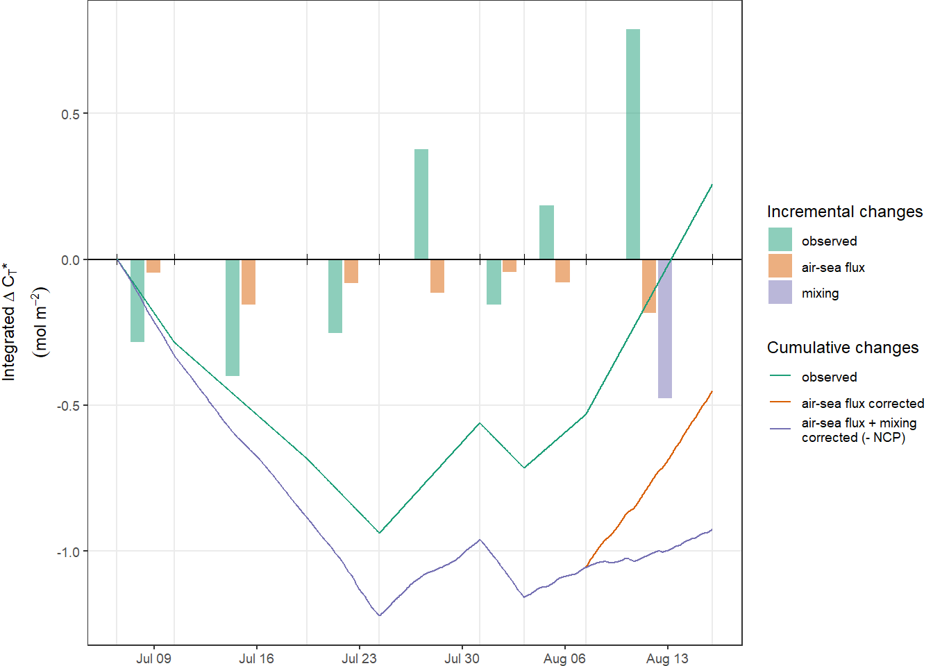
10.4 Write NCP files
NCP_flux_mix %>%
  write_csv(
    here::here(
      "data/intermediate/_merged_data_files/NCP_best_guess",
      "tm_NCP_cum.csv"
    )
  )

NCP_flux_mix_diff %>%
  write_csv(
    here::here(
      "data/intermediate/_merged_data_files/NCP_best_guess",
      "tm_NCP_inc.csv"
    )
  )
sessionInfo()R version 4.0.3 (2020-10-10)
Platform: x86_64-w64-mingw32/x64 (64-bit)
Running under: Windows 10 x64 (build 19042)
Matrix products: default
locale:
[1] LC_COLLATE=English_Germany.1252 LC_CTYPE=English_Germany.1252
[3] LC_MONETARY=English_Germany.1252 LC_NUMERIC=C
[5] LC_TIME=English_Germany.1252
attached base packages:
[1] grid stats graphics grDevices utils datasets methods
[8] base
other attached packages:
[1] ggsn_0.5.0 ggnewscale_0.4.5 rgdal_1.5-18
[4] LakeMetabolizer_1.5.0 rLakeAnalyzer_1.11.4.1 kableExtra_1.3.1
[7] sp_1.4-4 tibbletime_0.1.6 zoo_1.8-8
[10] lubridate_1.7.9.2 scico_1.2.0 metR_0.9.0
[13] marelac_2.1.10 shape_1.4.5 seacarb_3.2.14
[16] oce_1.2-0 gsw_1.0-5 testthat_3.0.1
[19] patchwork_1.1.1 forcats_0.5.0 stringr_1.4.0
[22] dplyr_1.0.2 purrr_0.3.4 readr_1.4.0
[25] tidyr_1.1.2 tibble_3.0.4 ggplot2_3.3.3
[28] tidyverse_1.3.0 workflowr_1.6.2
loaded via a namespace (and not attached):
[1] colorspace_2.0-0 rjson_0.2.20 ellipsis_0.3.1
[4] class_7.3-17 rprojroot_2.0.2 fs_1.5.0
[7] rstudioapi_0.13 farver_2.0.3 fansi_0.4.1
[10] xml2_1.3.2 codetools_0.2-16 knitr_1.30
[13] jsonlite_1.7.2 broom_0.7.5 dbplyr_2.0.0
[16] png_0.1-7 compiler_4.0.3 httr_1.4.2
[19] backports_1.2.1 assertthat_0.2.1 cli_2.2.0
[22] later_1.1.0.1 htmltools_0.5.0 tools_4.0.3
[25] ggmap_3.0.0 gtable_0.3.0 glue_1.4.2
[28] Rcpp_1.0.5 cellranger_1.1.0 raster_3.4-5
[31] vctrs_0.3.6 xfun_0.19 ps_1.5.0
[34] rvest_0.3.6 lifecycle_0.2.0 scales_1.1.1
[37] hms_0.5.3 promises_1.1.1 RColorBrewer_1.1-2
[40] yaml_2.2.1 stringi_1.5.3 highr_0.8
[43] maptools_1.0-2 e1071_1.7-4 checkmate_2.0.0
[46] RgoogleMaps_1.4.5.3 rlang_0.4.10 pkgconfig_2.0.3
[49] bitops_1.0-6 evaluate_0.14 lattice_0.20-41
[52] sf_0.9-6 labeling_0.4.2 tidyselect_1.1.0
[55] here_1.0.1 plyr_1.8.6 magrittr_2.0.1
[58] R6_2.5.0 generics_0.1.0 DBI_1.1.0
[61] pillar_1.4.7 haven_2.3.1 whisker_0.4
[64] foreign_0.8-80 withr_2.3.0 units_0.6-7
[67] modelr_0.1.8 crayon_1.3.4 KernSmooth_2.23-17
[70] utf8_1.1.4 rmarkdown_2.6 jpeg_0.1-8.1
[73] isoband_0.2.3 readxl_1.3.1 data.table_1.13.6
[76] git2r_0.27.1 reprex_0.3.0 digest_0.6.27
[79] classInt_0.4-3 webshot_0.5.2 httpuv_1.5.4
[82] munsell_0.5.0 viridisLite_0.3.0