Last updated: 2021-05-18

Checks: 7 0

Knit directory: BloomSail/

This reproducible R Markdown analysis was created with workflowr (version 1.6.2). The Checks tab describes the reproducibility checks that were applied when the results were created. The Past versions tab lists the development history.

R Markdown file: up-to-date

Great! Since the R Markdown file has been committed to the Git repository, you know the exact version of the code that produced these results.

Environment: empty

Great job! The global environment was empty. Objects defined in the global environment can affect the analysis in your R Markdown file in unknown ways. For reproduciblity it’s best to always run the code in an empty environment.

Seed: set.seed(20191021)

The command set.seed(20191021) was run prior to running the code in the R Markdown file. Setting a seed ensures that any results that rely on randomness, e.g. subsampling or permutations, are reproducible.

Session information: recorded

Great job! Recording the operating system, R version, and package versions is critical for reproducibility.

Cache: none

Nice! There were no cached chunks for this analysis, so you can be confident that you successfully produced the results during this run.

File paths: relative

Great job! Using relative paths to the files within your workflowr project makes it easier to run your code on other machines.

Repository version: 00a2574

Great! You are using Git for version control. Tracking code development and connecting the code version to the results is critical for reproducibility.

The results in this page were generated with repository version 00a2574. See the Past versions tab to see a history of the changes made to the R Markdown and HTML files.

Note that you need to be careful to ensure that all relevant files for the analysis have been committed to Git prior to generating the results (you can use wflow_publish or wflow_git_commit). workflowr only checks the R Markdown file, but you know if there are other scripts or data files that it depends on. Below is the status of the Git repository when the results were generated:


Ignored files:
    Ignored:    .Rhistory
    Ignored:    .Rproj.user/
    Ignored:    data/
    Ignored:    output/Plots/Figures_publication/.tmp.drivedownload/

Untracked files:
    Untracked:  data_os-2020-120_submission.zip

Unstaged changes:
    Modified:   code/Workflowr_project_managment.R
    Modified:   output/Plots/Figures_publication/Appendix/Fig_A1.pdf
    Modified:   output/Plots/Figures_publication/Appendix/Fig_A1.png
    Modified:   output/Plots/Figures_publication/Appendix/Fig_A2.pdf
    Modified:   output/Plots/Figures_publication/Appendix/Fig_B1.pdf
    Modified:   output/Plots/Figures_publication/Appendix/Fig_B1.png
    Modified:   output/Plots/Figures_publication/Appendix/Fig_B2.pdf
    Modified:   output/Plots/Figures_publication/Appendix/Fig_B2.png
    Modified:   output/Plots/Figures_publication/Appendix/Fig_C1.pdf
    Modified:   output/Plots/Figures_publication/Appendix/Fig_C2.pdf
    Modified:   output/Plots/Figures_publication/Appendix/Fig_C3.pdf
    Modified:   output/Plots/Figures_publication/Appendix/Fig_C3.png
    Modified:   output/Plots/Figures_publication/Appendix/Fig_C4.pdf
    Modified:   output/Plots/Figures_publication/Article/Fig_1.pdf
    Modified:   output/Plots/Figures_publication/Article/Fig_1.png
    Modified:   output/Plots/Figures_publication/Article/Fig_2.pdf
    Modified:   output/Plots/Figures_publication/Article/Fig_2.png
    Modified:   output/Plots/Figures_publication/Article/Fig_3.pdf
    Modified:   output/Plots/Figures_publication/Article/Fig_3.png
    Modified:   output/Plots/Figures_publication/Article/Fig_4.pdf
    Modified:   output/Plots/Figures_publication/Article/Fig_5.pdf
    Modified:   output/Plots/Figures_publication/Article/Fig_6.pdf
    Modified:   output/Plots/NCP_best_guess/tm_profiles_ID_pCO2_tem_sal_CT.pdf
    Modified:   output/Plots/NCP_best_guess/tm_profiles_pCO2_tem_sal_CT.pdf
    Modified:   output/Plots/response_time/all_plots.pdf
    Modified:   output/Plots/response_time/profiles_pCO2.pdf
    Modified:   output/Plots/response_time/profiles_pCO2_delta_grid.pdf
    Modified:   output/Plots/response_time/profiles_pCO2_delta_rel_grid.pdf
    Modified:   output/Plots/response_time/profiles_pCO2_grid.pdf
    Modified:   output/Plots/response_time/tau_determination_pCO2_corr_flushperiods_nls.pdf
    Modified:   output/Plots/response_time/time_series_depth_pCO2_corr_by_profile.pdf

Note that any generated files, e.g. HTML, png, CSS, etc., are not included in this status report because it is ok for generated content to have uncommitted changes.

These are the previous versions of the repository in which changes were made to the R Markdown (analysis/read-in.Rmd) and HTML (docs/read-in.html) files. If you’ve configured a remote Git repository (see ?wflow_git_remote), click on the hyperlinks in the table below to view the files as they were in that past version.

File	Version	Author	Date	Message
html	00a2574	jens-daniel-mueller	2021-05-10	Build site.
html	61e452c	jens-daniel-mueller	2021-04-16	Build site.
html	5f4fb9a	jens-daniel-mueller	2021-02-20	Build site.
html	6b47f30	jens-daniel-mueller	2021-02-20	Build site.
Rmd	5009016	jens-daniel-mueller	2021-02-20	cleaning
html	516b294	jens-daniel-mueller	2021-02-18	Build site.
html	70a8950	jens-daniel-mueller	2021-02-11	Build site.
html	4dfc4f8	jens-daniel-mueller	2021-02-11	Build site.
Rmd	8dc3356	jens-daniel-mueller	2021-02-11	cleaning
html	8e5e6d9	jens-daniel-mueller	2021-02-11	Build site.
Rmd	40f9a07	jens-daniel-mueller	2021-02-11	cleaning
html	8051798	jens-daniel-mueller	2021-02-10	Build site.
Rmd	9477a18	jens-daniel-mueller	2021-02-10	rerun all with empty folders
html	ed2a1b2	jens-daniel-mueller	2021-02-08	Build site.
Rmd	833d0f6	jens-daniel-mueller	2021-02-08	code and output cleaning
html	7027b12	jens-daniel-mueller	2021-02-08	Build site.
Rmd	3d6eaa1	jens-daniel-mueller	2021-02-08	code and output cleaning
html	c5fc34c	jens-daniel-mueller	2021-01-22	Build site.
html	4277235	jens-daniel-mueller	2021-01-05	Build site.
html	9a3f42a	jens-daniel-mueller	2020-10-24	Build site.
html	05248bf	jens-daniel-mueller	2020-10-20	Build site.
html	1c4fe8e	jens-daniel-mueller	2020-10-20	table with time series in depth intervals added
html	a43fcac	jens-daniel-mueller	2020-10-13	Build site.
Rmd	a23fb5d	jens-daniel-mueller	2020-10-13	removed unnecessary output prints
html	6896725	jens-daniel-mueller	2020-10-01	Build site.
Rmd	f2f9226	jens-daniel-mueller	2020-10-01	tower data converted to UTC
html	9f66019	jens-daniel-mueller	2020-10-01	Build site.
html	27c5431	jens-daniel-mueller	2020-09-29	Build site.
Rmd	2e0f902	jens-daniel-mueller	2020-09-29	all parameters separate, rebuild
html	1d01685	jens-daniel-mueller	2020-09-28	Build site.
Rmd	d28129f	jens-daniel-mueller	2020-09-28	republish after tau factor set to 1 and using final pCO2 data
html	02a1609	jens-daniel-mueller	2020-09-25	Build site.
Rmd	99e69cf	jens-daniel-mueller	2020-09-25	activated read-in of th and ts data
Rmd	616c27f	jens-daniel-mueller	2020-09-25	updated repo manually
html	904f0f7	jens-daniel-mueller	2020-09-23	Build site.
html	66bf52a	jens-daniel-mueller	2020-09-23	Build site.
Rmd	0c8eed6	jens-daniel-mueller	2020-09-23	included postprocessed cleaned data
html	c919fb7	jens-daniel-mueller	2020-06-29	Build site.
Rmd	1461cb6	jens-daniel-mueller	2020-06-29	Fig update for talk
html	603af23	jens-daniel-mueller	2020-05-25	Build site.
html	3414c23	jens-daniel-mueller	2020-05-25	Build site.
html	9ccd9a3	jens-daniel-mueller	2020-05-25	Build site.
Rmd	9bedac5	jens-daniel-mueller	2020-05-25	revised pp time series plot
html	dd3bd89	jens-daniel-mueller	2020-05-07	Build site.
Rmd	ad98da2	jens-daniel-mueller	2020-05-07	harmonized parameter labeling
html	3832733	jens-daniel-mueller	2020-04-30	Build site.
Rmd	4f4ab08	jens-daniel-mueller	2020-04-30	harmonized code until RT determination
html	1b6480f	jens-daniel-mueller	2020-04-30	Build site.
Rmd	fe72316	jens-daniel-mueller	2020-04-30	revised variable and object names, used temp-dependent tau only, rerun code
html	d9248a6	jens-daniel-mueller	2020-04-29	Build site.
Rmd	70bd3f0	jens-daniel-mueller	2020-04-29	correct interpolation, new d pco2 plot
html	aa52c73	jens-daniel-mueller	2020-04-28	Build site.
Rmd	3044ec0	jens-daniel-mueller	2020-04-28	completely revised
html	57f7231	jens-daniel-mueller	2020-04-28	Build site.
Rmd	5ebd364	jens-daniel-mueller	2020-04-28	revised
html	b5722a7	jens-daniel-mueller	2020-04-28	Build site.
html	472c2b4	jens-daniel-mueller	2020-04-21	Build site.
html	f8fcf50	jens-daniel-mueller	2020-04-19	created pub figures for time series
html	87658c3	jens-daniel-mueller	2020-04-14	Build site.
Rmd	5c96a65	jens-daniel-mueller	2020-04-14	temperature penetration depth
html	624835e	jens-daniel-mueller	2020-04-02	Build site.
Rmd	a7ac65d	jens-daniel-mueller	2020-04-02	BloomSail data 1-5m and sd in time series plots
html	26cf733	jens-daniel-mueller	2020-04-02	Build site.
Rmd	57b77af	jens-daniel-mueller	2020-04-02	corrected Finnmaid lat borders and plotted fm track in map
html	a6c4c22	jens-daniel-mueller	2020-03-30	Build site.
html	80c78b3	jens-daniel-mueller	2020-03-30	Build site.
html	5f8ca30	jens-daniel-mueller	2020-03-20	Build site.
Rmd	1ebd01a	jens-daniel-mueller	2020-03-20	reorganitzed filenames and navbar

library(tidyverse)
library(data.table)
library(lubridate)
library(DataExplorer)
library(leaflet)
library(readxl)
library(gsubfn)

1 Scope of this script

For each data source:

read raw data files
harmonize column names
clean obvious erroneous data
merged into one file
write merged file

2 Sea-Bird SBE 16 sensor data (ts)

CTD sensor data including recordings from the analog output of auxiliary pH, O₂, Chla and pCO₂ sensors were recorded with a measurement frequency of 15 sec. (In addition, pCO₂ data were also internally recorded on the Contros HydroC instrument with higher temporal resolution and will later be used for further analysis after merging with CTD data.)

2.1 Read regular profiles and transects

files <-
  list.files(path = "data/input/TinaV/Sensor/Profiles_Transects/", pattern = "[.]cnv$")

for (file in files) {
  start_date <-
    data.table(read.delim(
      here::here("data/input/TinaV/Sensor/Profiles_Transects/", file),
      sep = "#",
      nrows = 160
    ))[[78, 1]]
  start_date <- substr(start_date, 15, 34)
  start_date <- mdy_hms(start_date, tz = "UTC")
  
  temp <-
    read.delim(
      here::here("data/input/TinaV/Sensor/Profiles_Transects/", file),
      sep = "",
      skip = 160,
      header = FALSE
    )
  temp <- data.table(temp[, c(2, 3, 4, 5, 6, 7, 9, 11, 13)])
  names(temp) <-
    c("date_time",
      "dep",
      "tem",
      "sal",
      "V_pH",
      "pH",
      "Chl",
      "O2",
      "pCO2_analog")
  temp$start_date <- start_date
  temp$date_time <- temp$date_time + temp$start_date
  
  temp$ID <- substr(file, 1, 6)
  temp$type <- substr(file, 8, 8)
  temp$station <- substr(file, 8, 10)
  
  temp$cast <- "up"
  temp[date_time < mean(temp[dep == max(temp$dep)]$date_time)]$cast <-
    "down"
  
  if (exists("dataset")) {
    dataset <- rbind(dataset, temp)
  }
  
  if (!exists("dataset")) {
    dataset <- temp
  }
  
  rm(start_date)
  rm(temp)
}


ts <- dataset
rm(dataset, file, files)

2.2 Read profiles and transects around Östergarnsholm

files <-
  list.files(path = "data/input/TinaV/Sensor/Ostergarnsholm/", pattern = "[.]cnv$")

for (file in files) {
  start_date <-
    data.table(read.delim(
      here::here("data/input/TinaV/Sensor/Ostergarnsholm/", file),
      sep = "#",
      nrows = 160
    ))[[78, 1]]
  start_date <- substr(start_date, 15, 34)
  start_date <- mdy_hms(start_date, tz = "UTC")
  
  temp <-
    read.delim(
      here::here("data/input/TinaV/Sensor/Ostergarnsholm/", file),
      sep = "",
      skip = 160,
      header = FALSE
    )
  temp <- data.table(temp[, c(2, 3, 4, 5, 6, 7, 9, 11, 13)])
  names(temp) <-
    c("date_time",
      "dep",
      "tem",
      "sal",
      "V_pH",
      "pH",
      "Chl",
      "O2",
      "pCO2_analog")
  temp$start_date <- start_date
  temp$date_time <- temp$date_time + temp$start_date
  
  temp$ID <- substr(file, 1, 6)
  temp$type <- substr(file, 8, 8)
  temp$station <- substr(file, 11, 12)
  
  temp$cast <- "up"
  temp[date_time < mean(temp[dep == max(temp$dep)]$date_time)]$cast <-
    "down"
  
  if (exists("dataset")) {
    dataset <- rbind(dataset, temp)
  }
  
  if (!exists("dataset")) {
    dataset <- temp
  }
  
  rm(start_date)
  rm(temp)
}


ts_OGB <- dataset
rm(dataset, file, files)

ts_OGB <- ts_OGB %>%
  mutate(
    type = if_else(station == "bo", "P", "T"),
    station = if_else(station == "bo", "P14", station),
    station = if_else(station == "in", "T14", station),
    station = if_else(station == "ou", "T15", station)
  )

ts <- bind_rows(ts, ts_OGB) %>%
  arrange(date_time)

rm(ts_OGB)

2.3 EDA raw data

source("code/eda.R")
eda(ts, "ts-raw")
rm(eda)

The output of an automated Exploratory Data Analysis (EDA) performed on the raw data with the package DataExplorer can be accessed here:

Link to EDA report of CTD raw data

2.4 Clean data set

Sensor recordings were cleaned from obviously erroneous readings, by setting suspicious values to NA.

# running the commented code for plotting
# before and after the cleaning steps
# allows to visualize the removal of errorneous readings

ts <- data.table(ts)

# Profiling data

# temperature

# ts %>%
#   filter(type == "P") %>%
#   ggplot(aes(tem, dep, col=station, linetype = cast))+
#   geom_line()+
#   scale_y_reverse()+
#   geom_vline(xintercept = c(10, 20))+
#   facet_wrap(~ID)

ts[ID == "180723" & station == "P07" & dep < 2 & cast == "up"]$tem <- NA

# salinity

# ts %>%
#   filter(type == "P") %>%
#   ggplot(aes(sal, dep, col=station, linetype = cast))+
#   geom_path()+
#   scale_y_reverse()+
#   facet_wrap(~ID)

ts[sal < 6]$sal <- NA

# pH

# ts %>%
#   filter(type == "P") %>%
#   ggplot(aes(pH, dep, col=station, linetype=cast))+
#   geom_path()+
#   scale_y_reverse()+
#   facet_wrap(~ID)
# 
# ts %>%
#   filter(type == "P") %>%
#   ggplot(aes(V_pH, dep, col=station, linetype=cast))+
#   geom_path()+
#   scale_y_reverse()+
#   facet_wrap(~ID)

ts[pH < 7.5]$V_pH <- NA
ts[pH < 7.5]$pH <- NA

ts[ID == "180709" & station == "P03" & dep < 5 & cast == "down"]$pH <- NA
ts[ID == "180709" & station == "P05" & dep < 10 & cast == "down"]$pH <- NA
ts[ID == "180718" & station == "P10" & dep < 3 & cast == "down"]$pH <- NA
ts[ID == "180815" & station == "P03" & dep < 2 & cast == "down"]$pH <- NA
ts[ID == "180820" & station == "P11" & dep < 15 & cast == "down"]$pH <- NA

ts[ID == "180709" & station == "P03" & dep < 5 & cast == "down"]$V_pH <- NA
ts[ID == "180709" & station == "P05" & dep < 10 & cast == "down"]$V_pH <- NA
ts[ID == "180718" & station == "P10" & dep < 3 & cast == "down"]$V_pH <- NA
ts[ID == "180815" & station == "P03" & dep < 2 & cast == "down"]$V_pH <- NA
ts[ID == "180820" & station == "P11" & dep < 15 & cast == "down"]$V_pH <- NA


# pCO2

# ts %>%
#   filter(type == "P") %>%
#   ggplot(aes(pCO2, dep, col=station, linetype = cast))+
#   geom_path()+
#   scale_y_reverse()+
#   facet_wrap(~ID)

ts[ID == "180616"]$pCO2_analog <- NA

# O2

# ts %>% 
#   filter(type == "P") %>% 
#   ggplot(aes(O2, dep, col=station, linetype = cast))+
#   geom_path()+
#   scale_y_reverse()+
#   facet_wrap(~ID)

# Chlorophyll

# ts %>%
#   filter(type == "P") %>%
#   ggplot(aes(Chl, dep, col=station, linetype = cast))+
#   geom_path()+
#   scale_y_reverse()+
#   facet_wrap(~ID)

ts[Chl > 100]$Chl <- NA


# Surface transect data

# ts %>%
#   filter(type == "T") %>%
#   ggplot(aes(date, dep, col=station))+
#   geom_point()+
#   scale_y_reverse()+
#   facet_wrap(~ID, scales = "free_x")
# 
# ts %>%
#   filter(type == "T") %>%
#   ggplot(aes(date, tem, col=station))+
#   geom_point()+
#   facet_wrap(~ID, scales = "free_x")
# 
# ts %>%
#   filter(type == "T") %>%
#   ggplot(aes(date, sal, col=station))+
#   geom_point()+
#   facet_wrap(~ID, scales = "free_x")
# 
# ts %>%
#   filter(type == "T") %>%
#   ggplot(aes(date, pCO2, col=station))+
#   geom_point()+
#   facet_wrap(~ID, scales = "free_x")
# 
# ts %>%
#   filter(type == "T") %>%
#   ggplot(aes(date, pH, col=station))+
#   geom_point()+
#   facet_wrap(~ID, scales = "free_x")
# 
# ts %>%
#   filter(type == "T") %>%
#   ggplot(aes(date, Chl, col=station))+
#   geom_point()+
#   facet_wrap(~ID, scales = "free_x")

ts[type == "T" & Chl > 10]$Chl <- NA


# ts %>% 
#   filter(type == "T") %>% 
#   ggplot(aes(date, O2, col=station))+
#   geom_point()+
#   facet_wrap(~ID, scales = "free_x")

2.5 Write summary file

Relevant columns were selected and renamed, only observations from regular stations (P01-P13) and transects (T01-T13) were selected and summarized data were written to file.

ts <- ts %>% 
  select(date_time,
         ID,
         type,
         station,
         dep,
         sal,
         tem,
         pCO2_analog)

ts %>% 
  write_csv(here::here("data/intermediate/_summarized_data_files", "ts.csv"))

2.6 EDA clean data

source("code/eda.R")
eda(ts, "ts_clean")

rm(eda)

The output of an automated Exploratory Data Analysis (EDA) performed on the cleaned data with the package DataExplorer can be accessed here:

Link to EDA report of CTD clean data

2.7 Overview plots

ts %>%
  arrange(date_time) %>%
  filter(type == "P",!(station %in% c("PX1", "PX2"))) %>%
  ggplot(aes(tem, dep, col = ymd(ID), group = ID)) +
  geom_path() +
  scale_y_reverse() +
  scale_color_viridis_c(trans = "date", name = "") +
  facet_wrap( ~ station)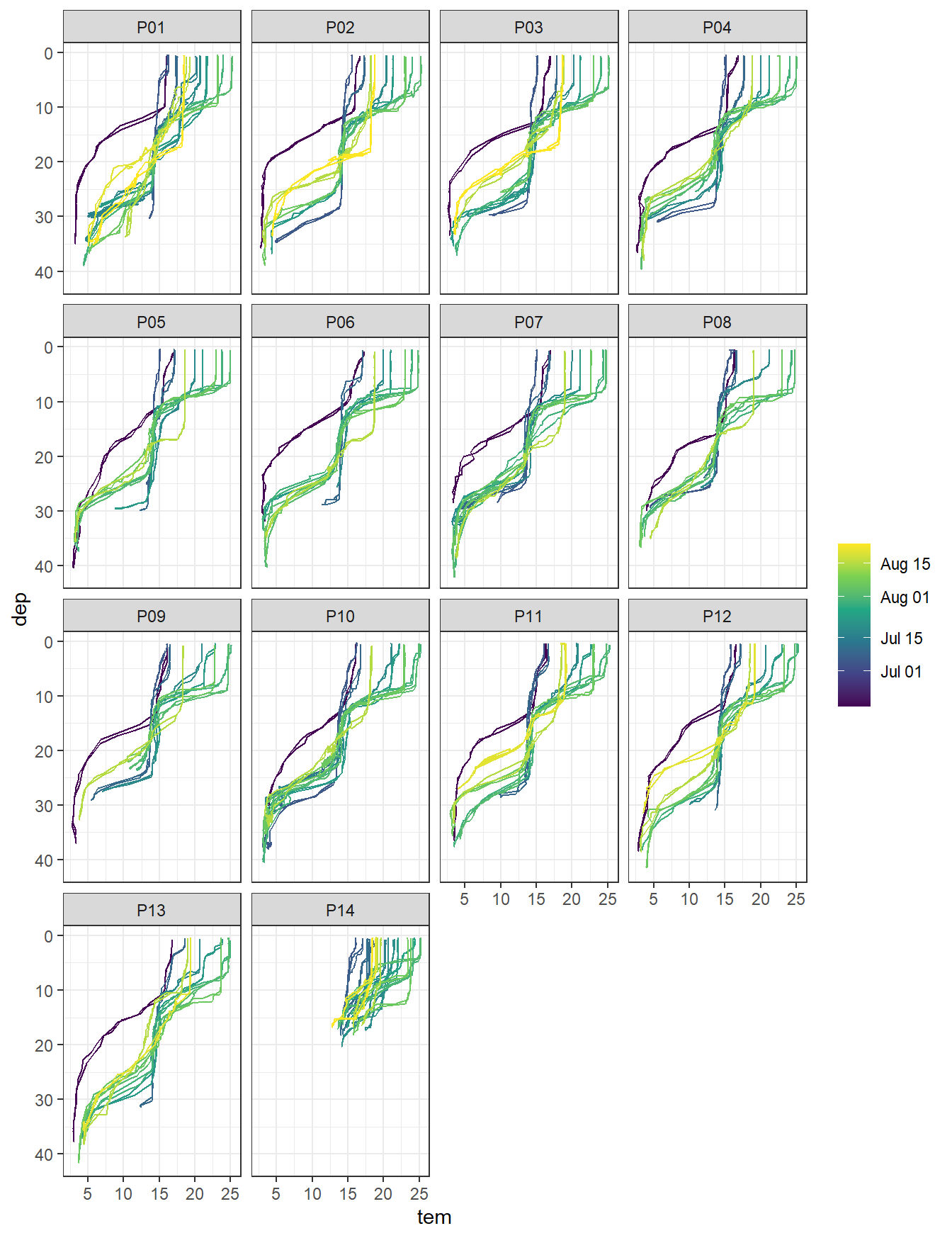

Temperature profiles by stations. Color refers to the starting date of each cruise.

ts %>%
  arrange(date_time) %>%
  filter(type == "P",!(station %in% c("PX1", "PX2"))) %>%
  ggplot(aes(pCO2_analog, dep, col = ymd(ID), group = ID)) +
  geom_path() +
  scale_y_reverse() +
  scale_color_viridis_c(trans = "date", name = "") +
  facet_wrap( ~ station)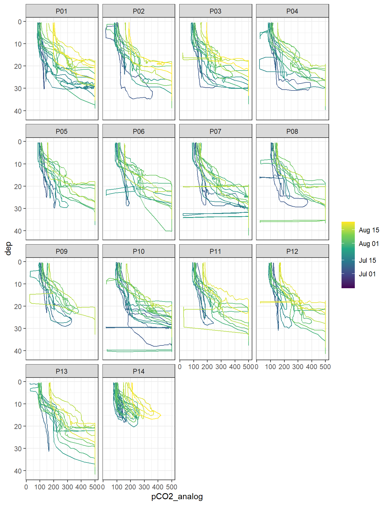

pCO~2~ (analog signal) profiles by stations. Color refers to the starting date of each cruise.

pCO₂ (analog signal) profiles by stations. Color refers to the starting date of each cruise.

3 HydroC CO₂ data (th)

3.1 Read data

Originally, HydroC pCO₂ data were provided by KM Contros after applying a drift correction to the raw data, which was based on pre- and post-deployment calibration results. Those preliminary data are read-in here and referred to as V1. However, some data recorded during testing and configuration of the sensor were later on removed, and the post-processing was repeated based on a cleaned data set. This revised post-processed file is referred to as V2 and used in the merging script.

# Read Contros corrected data file, based on all recordings
th <-
  read_csv2(here::here("data/input/TinaV/Sensor/HydroC-pCO2/corrected_Contros",
                       "parameter&pCO2s(method 43).txt"),
            col_names = c("date_time", "Zero", "Flush", "p_NDIR",
                          "p_in", "T_control", "T_gas", "%rH_gas",
                          "Signal_raw", "Signal_ref", "T_sensor",
                          "pCO2_corr", "Runtime", "nr.ave")) %>% 
  mutate(date_time = dmy_hms(date_time),
         Flush = as.factor(as.character(Flush)),
         Zero = as.factor(as.character(Zero)))

3.2 Deployment identification and subsetting

Individual deployments (periods of observations with less than 30 sec between recordings) were identified and relevant deployment periods were selected. This procedure removes some data recorded during sensor testing and set-up.

# identify individual deployments
th <- th %>%
  arrange(date_time) %>%
  mutate(deployment = cumsum(c(TRUE, diff(date_time) >= 30)))

# write pre-cleaning file for later comparison
th %>%
  select(date_time, pCO2_corr, deployment) %>%
  write_csv(here::here(
    "data/intermediate/_summarized_data_files",
    "th_pre_cleaning.csv"
  ))

# filter relevant deployments
th <- th %>%
  filter(deployment %in% c(2, 6, 9, 14, 17, 21, 23, 27, 31, 33, 34, 35, 37))

3.3 Removal of duplicated time stamps

A low number of the recorded HydroC data revealed the exact same time stamp. This was corrected either by filling a corresponding gap before or after the duplicate, or by removing one of the duplicated rows if no such gap existed.

# add counter for date_time observations
th <- th %>%
  add_count(date_time)

# find triplicated time stamp and select only first observation, and merge

th_no_triple <- th %>%
  filter(n <= 2)

th_triple_clean <- th %>%
  filter(n > 2) %>%
  slice(1)

th <- full_join(th_no_triple, th_triple_clean)

rm(list = setdiff(ls(), c("th", "parameters")))


# find duplicated time stamps and shift first by one second backward, and merge

# th %>%
#   distinct(date_time)

th <- th %>%
  select(-n) %>%
  add_count(date_time)

# unique(th$n)

th_no_duplicated <- th %>%
  filter(n == 1)

th_duplicated <- th %>%
  filter(n == 2)

th_duplicated_first <- th_duplicated %>%
  group_by(date_time) %>%
  slice(1) %>%
  ungroup() %>%
  mutate(date_time = date_time - 1)

th_duplicated_second <- th_duplicated %>%
  group_by(date_time) %>%
  slice(2) %>%
  ungroup()

th_duplicated_clean <-
  full_join(th_duplicated_first, th_duplicated_second) %>%
  arrange(date_time)

th <- full_join(th_no_duplicated, th_duplicated_clean)

# th %>%
#   distinct(date_time)

rm(list = setdiff(ls(), c("th", "parameters")))



# find duplicated time stamps and shift first by two seconds forward, and merge

# th %>%
#   distinct(date_time)

th <- th %>%
  select(-n) %>%
  add_count(date_time)

# unique(th$n)

th_no_duplicated <- th %>%
  filter(n == 1)

th_duplicated <- th %>%
  filter(n == 2)

th_duplicated_first <- th_duplicated %>%
  group_by(date_time) %>%
  slice(1) %>%
  ungroup() %>%
  mutate(date_time = date_time + 2)

th_duplicated_second <- th_duplicated %>%
  group_by(date_time) %>%
  slice(2) %>%
  ungroup()

th_duplicated_clean <-
  full_join(th_duplicated_first, th_duplicated_second) %>%
  arrange(date_time)

th <- full_join(th_no_duplicated, th_duplicated_clean)

# th %>%
#   distinct(date_time)

rm(list = setdiff(ls(), c("th", "parameters")))

# remaining duplicates are observations where other observations with a +/- 1 sec timestamp exist
# for those cases, only the first duplicated observation is selected (similar to triplicate treatment)


# th %>%
#   distinct(date_time)

th <- th %>%
  select(-n) %>%
  add_count(date_time)

# unique(th$n)


th_still_no_duplicated <- th %>%
  filter(n == 1)

th_still_duplicated_first <- th %>%
  filter(n == 2) %>%
  group_by(date_time) %>%
  slice(1)

th <- full_join(th_still_no_duplicated, th_still_duplicated_first)

# th %>%
#   distinct(date_time)

rm(list = setdiff(ls(), c("th", "parameters")))

th <- th %>%
  select(-n)

3.4 Flush and Zeroing identification

Flush and zeroing periods of the sensor are identified and assigned with unique IDs.

# Zeroing ID labeling

th <- th %>%
  arrange(date_time) %>%
  group_by(Zero) %>%
  mutate(Zero_counter = as.factor(cumsum(c(
    TRUE, diff(date_time) >= 30
  )))) %>%
  ungroup()

# Flush: Identification

th <- th %>%
  mutate(Flush = 0) %>%
  group_by(Zero, Zero_counter) %>%
  mutate(
    start = min(date_time),
    duration = date_time - start,
    Flush = if_else(Zero == 0 &
                      duration < parameters$HC_flush_duration, "1", "0")
  ) %>%
  ungroup()


#  Flush: Identify equilibration and internal gas mixing periods

th <- th %>%
  mutate(mixing = if_else(
    duration < parameters$HC_mixing_duration,
    "mixing",
    "equilibration"
  ))

3.5 Deployment plots

pdf(
  file = here::here("output/Plots/read_in",
                    "th_deployments.pdf"),
  onefile = TRUE,
  width = 7,
  height = 4
)

for (i in unique(th$deployment)) {
  sub <-  th %>%
    filter(deployment == i)
  start_date <- min(sub$date_time)
  
  print(sub %>%
          ggplot(aes(date_time, pCO2_corr, col = Zero_counter)) +
          geom_line() +
          labs(title = paste(
            "Deployment: ", i, "| Start time: ", start_date
          )))
  
}

dev.off()

rm(sub, start_date, i)

A pdf with pCO₂ timeseries plots of all individual deployments can be found here:

Link to pCO₂ timeseries plots

source("code/eda.R")
eda(th, "th")
rm(eda)

The output of an automated Exploratory Data Analysis (EDA) performed with the package DataExplorer can be accessed here:

Link to EDA report of HydroC pCO₂ data data

3.6 Write summary file

Summarized clean pCO₂ data were written to file.

th %>%
  select(date_time,
         Zero,
         Flush,
         pCO2_corr,
         deployment,
         Zero_counter,
         duration,
         mixing) %>%
  write_csv(here::here("data/intermediate/_summarized_data_files",
                       "th.csv"))

rm(th)

4 Bottle data CO₂ (tb)

Discrete samples were collected with a Niskin bottle and analyzed for CT and AT at IOW’s CO₂ lab.

4.1 Read data

# Read CO2 system bottle data
tb <-
  read_csv(
    here::here(
      "data/input/TinaV/Bottle/Tracegases",
      "BloomSail_bottle_CO2_all.csv"
    ),
    col_types = list("c", "c", "n", "n", "n", "n", "n")
  )

# select and rename relevant columns
tb <- tb %>%
  select(
    ID = transect.ID,
    station = label,
    dep = Dep,
    sal = Sal,
    CT,
    AT
  )

4.2 Write summary file

tb %>% write_csv(here::here("data/intermediate/_summarized_data_files",
                            "tb.csv"))
rm(tb)

5 Bottle data plankton (tp)

Discrete samples were collected with a Niskin bottle and analysed for phytoplankton composition and biomass at IOW’s phytoplankton lab (Norbert Wasmund).

5.1 Read data

tp <- read_csv(
  here::here(
    "data/input/TinaV/Bottle/Phytoplankton",
    "181205_BloomSail_Plankton_counts.csv"
  )
)

# delete colomns that contain counts, not calculated biomass
tp <- tp[, -seq(4, 21, 1)]

# assign new column names
# for species: 
# nr = size class, 
# HV = Heterocyst per Volume, 
# Hl = Heterocyst per length, 
# t = total

names(tp) <-
  c(
    "date",
    "station",
    "dep",
    "Aphanizomenon.1",
    "Aphanizomenon.2",
    "Aphanizomenon.3",
    "Aphanizomenon.t",
    "Aphanizomenon.HV",
    "Aphanizomenon.Hl",
    "Dolichospermum.1",
    "Dolichospermum.2",
    "Dolichospermum.3",
    "Dolichospermum.4",
    "Dolichospermum.t",
    "Dolichospermum.HV",
    "Dolichospermum.Hl",
    "Nodularia.1",
    "Nodularia.2",
    "Nodularia.3",
    "Nodularia.t",
    "Nodularia.HV",
    "Nodularia.Hl",
    "Nodulariadead.1",
    "Nodulariadead.2",
    "Nodulariadead.3",
    "Nodulariadead.t",
    "total.t"
  )


# change format of data table and separate into 2 columns for species and class

tp <-
  gather(tp, para, value, Aphanizomenon.1:total.t, factor_key = TRUE)

tp <- separate(tp, col = para, into = c("Species", "class"))

# change class of columns
tp <- tp %>%
  mutate(ID = date,
         date = ymd(date))

5.2 Write summary file

tp %>% write_csv(here::here("data/intermediate/_summarized_data_files",
                            "tp.csv"))
rm(tp)

6 GPS track (tt)

GPS track data were recorded with a Samsung Galaxy tablet.

6.1 Read data

files <-
  list.files(path = "data/input/TinaV/Track/GPS_Logger_Track/", pattern = "[.]txt$")

for (file in files) {
  # if the merged dataset does exist, append to it
  if (exists("dataset")) {
    temp <-
      data.table(read.delim(
        here::here("data/input/TinaV/Track/GPS_Logger_Track", file),
        sep = ","
      )[, c(2, 3, 4)])
    names(temp) <- c("date_time", "lat", "lon")
    temp$date_time <- ymd_hms(temp$date, tz = "UTC")
    
    dataset <- rbind(dataset, temp)
    rm(temp)
  }
  
  # if the merged dataset doesn't exist, create it
  if (!exists("dataset")) {
    dataset <-
      data.table(read.delim(
        here::here("data/input/TinaV/Track/GPS_Logger_Track", file),
        sep = ","
      )[, c(2, 3, 4)])
    names(dataset) <- c("date_time", "lat", "lon")
    dataset$date_time <- ymd_hms(dataset$date_time, tz = "UTC")
    
  }
}

tt <- dataset
rm(dataset, file, files)

6.2 Write summary file

tt %>%
  write_csv(here::here("data/intermediate/_summarized_data_files",
                       "tt.csv"))

rm(tt)

7 Atmospheric observations

Atmospheric data were recorded at the ICOS station on Östergarnsholm.

7.1 Read data

og <-
  read_delim(
    here::here(
      "data/input/Ostergarnsholm/Tower",
      "Oes_Jens_atm_water_June_to_August_2018.csv"
    ),
    delim = ";"
  )

og <- og %>%
  mutate(date_time = ymd_hms(paste(
    paste(year, month, day, sep = "/"),
    paste(hour, min, sec, sep = ":")
  ))) %>%
  select(
    "date_time",
    "CO2 12m [ppm]",
    "w_c [ppm m/s]",
    "WS 12m [m/s]",
    "WD 12m [degrees]",
    "T 12m [degrees C]",
    "RIS [W/m^2]"
  )

# conversion from GMT+1 to UTC
og <- og %>%
  mutate(date_time = date_time - 60 ^ 2)

og <- og %>%
  select(date_time, pCO2_atm = "CO2 12m [ppm]", wind = "WS 12m [m/s]")

7.2 Write summary file

og %>%
  write_csv(here::here("data/intermediate/_summarized_data_files",
                       "og.csv"))

rm(og)

8 SOOP Finnmaid

Here, we read in pCO₂ and SST data recorded on SOOP Finnmaid in June-August 2018.

8.1 Read data

# LI-COR data

files <-
  list.files(path = "data/input/Finnmaid_2018", pattern = "[.]xls$")

for (file in files) {
  temp <- read_excel(here::here("data/input/Finnmaid_2018", file))
  temp <- temp[c(1, 2, 3, 12, 7, 4, 15, 8, 5, 17)]
  names(temp) <-
    c("date_time",
      "lon",
      "lat",
      "pCO2",
      "sal",
      "tem",
      "cO2",
      "patm",
      "Teq",
      "xCO2")
  temp <- temp[-c(1), ]
  temp$date_time <-
    as.POSIXct(as.numeric(temp$date_time) * 60 * 60 * 24,
               origin = "1899-12-30",
               tz = "GMT")
  temp$lon <- as.numeric(as.character(temp$lon))
  temp$lat <- as.numeric(as.character(temp$lat))
  temp$pCO2 <- as.numeric(as.character(temp$pCO2))
  temp$sal <- as.numeric(as.character(temp$sal))
  temp$tem <- as.numeric(as.character(temp$tem))
  temp$cO2 <- as.numeric(as.character(temp$cO2))
  temp$patm <- as.numeric(as.character(temp$patm))
  temp$Teq <- as.numeric(as.character(temp$Teq))
  temp$xCO2 <- as.numeric(as.character(temp$xCO2))
  temp <- data.table(temp)
  
  temp$route <-
    strapplyc(as.character(file), ".*(.).xls*", simplify = TRUE)
  temp$ID <- substr(as.character(file), 3, 10)
  
  if (exists("dataset")) {
    dataset <- rbind(dataset, temp)
  } else{
    dataset <- temp
  }
  
}


rm(temp, files, file)
dataset <- dataset[pCO2 != 0]


# Los Gatos Research (LGR) data
# Please note that the LGR data were corrected manually before
# The correction procedure is outlined in the Appendix of the ms

files <-
  list.files(path = "data/input/Finnmaid_2018/LGR", pattern = "[.]xls$")

for (file in files) {
  temp <- read_excel(here::here("data/input/Finnmaid_2018/LGR", file))
  temp <- temp[c(2, 3, 4, 8, 6, 5, 14, 7, 15, 9)]
  names(temp) <-
    c("date_time",
      "lon",
      "lat",
      "pCO2",
      "sal",
      "tem",
      "cO2",
      "patm",
      "Teq",
      "xCO2")
  temp <- temp[-c(1), ]
  temp$date_time <- dmy_hms(temp$date_time)
  temp <- data.table(temp)
  
  temp$route <- substr(as.character(file), 12, 12)
  temp$ID <- substr(as.character(file), 3, 10)
  
  if (exists("dataset.LGR")) {
    dataset.LGR <- rbind(dataset.LGR, temp)
  } else{
    dataset.LGR <- temp
  }
  
}

rm(temp, files, file)

# This code can be used to convert O2 units
# but is not applied, because O2 data are not used in this study

source(here::here("code", "O2stoO2c.R"))

dataset.LGR <- dataset.LGR %>%
  filter() %>%
  mutate(cO2 = O2stoO2c(
    O2sat = cO2,
    T = tem,
    S = sal,
    P = 3 / 10,
    p_atm = 1013.5
  ))

rm(O2stoO2c, pH2Osat, sca_T, Scorr, TCorr, R, Vm)

dataset$sensor <- "LICOR"
dataset.LGR$sensor <- "LosGatos"

fm <- bind_rows(dataset, dataset.LGR)

rm(dataset, dataset.LGR)

8.2 Write summary file

fm %>% 
  write_csv(here::here("data/intermediate/_summarized_data_files",
                       "fm.csv"))
rm(fm)

9 Interactive map

fm <-
  read_csv(here::here("data/intermediate/_summarized_data_files",
                      "fm.csv"))

fm_sub <- fm %>%
  arrange(date_time) %>%
  slice(which(row_number() %% 20 == 1))

tt <-
  read_csv(here::here("data/intermediate/_summarized_data_files", "tt.csv"))

tt_sub <- tt %>%
  slice(which(row_number() %% 20 == 1))

rm(tt, fm)

leaflet() %>%
  setView(lng = 20, lat = 57.3, zoom = 8) %>%
  addLayersControl(
    baseGroups = c("Ocean Basemap",
                   "Satellite"),
    overlayGroups = c("BloomSail", "Finnmaid"),
    options = layersControlOptions(collapsed = FALSE),
    position = 'topright'
  ) %>%
  addProviderTiles("Esri.WorldImagery", group = "Satellite") %>%
  addProviderTiles(providers$Esri.OceanBasemap, group = "Ocean Basemap") %>%
  addScaleBar(position = 'topright') %>%
  addMeasure(
    primaryLengthUnit = "kilometers",
    secondaryLengthUnit = 'miles',
    primaryAreaUnit = "sqmeters",
    secondaryAreaUnit = "acres",
    position = 'topleft'
  ) %>%
  addCircles(data = fm_sub,
             ~ lon,
             ~ lat,
             color = "white",
             group = "Finnmaid") %>%
  addPolylines(data = tt_sub,
               ~ lon,
               ~ lat,
               color = "red",
               group = "BloomSail")

Overview map of SOOP Finnmaid and SV Tina V tracks. Please note that only a subet of the recorded track data is plotted.

rm(fm_sub, tt_sub)

sessionInfo()

R version 4.0.3 (2020-10-10)
Platform: x86_64-w64-mingw32/x64 (64-bit)
Running under: Windows 10 x64 (build 19042)

Matrix products: default

locale:
[1] LC_COLLATE=English_Germany.1252  LC_CTYPE=English_Germany.1252   
[3] LC_MONETARY=English_Germany.1252 LC_NUMERIC=C                    
[5] LC_TIME=English_Germany.1252    

attached base packages:
[1] stats     graphics  grDevices utils     datasets  methods   base     

other attached packages:
 [1] gsubfn_0.7         proto_1.0.0        readxl_1.3.1       leaflet_2.0.3     
 [5] DataExplorer_0.8.2 lubridate_1.7.9.2  data.table_1.13.6  forcats_0.5.0     
 [9] stringr_1.4.0      dplyr_1.0.2        purrr_0.3.4        readr_1.4.0       
[13] tidyr_1.1.2        tibble_3.0.4       ggplot2_3.3.3      tidyverse_1.3.0   
[17] workflowr_1.6.2   

loaded via a namespace (and not attached):
 [1] httr_1.4.2              jsonlite_1.7.2          viridisLite_0.3.0      
 [4] here_1.0.1              modelr_0.1.8            assertthat_0.2.1       
 [7] highr_0.8               cellranger_1.1.0        yaml_2.2.1             
[10] pillar_1.4.7            backports_1.2.1         glue_1.4.2             
[13] digest_0.6.27           promises_1.1.1          rvest_0.3.6            
[16] leaflet.providers_1.9.0 colorspace_2.0-0        htmltools_0.5.0        
[19] httpuv_1.5.4            pkgconfig_2.0.3         broom_0.7.5            
[22] haven_2.3.1             scales_1.1.1            whisker_0.4            
[25] later_1.1.0.1           git2r_0.27.1            generics_0.1.0         
[28] farver_2.0.3            ellipsis_0.3.1          withr_2.3.0            
[31] cli_2.2.0               magrittr_2.0.1          crayon_1.3.4           
[34] evaluate_0.14           ps_1.5.0                fs_1.5.0               
[37] fansi_0.4.1             xml2_1.3.2              tools_4.0.3            
[40] hms_0.5.3               lifecycle_0.2.0         munsell_0.5.0          
[43] reprex_0.3.0            networkD3_0.4           compiler_4.0.3         
[46] rlang_0.4.10            grid_4.0.3              rstudioapi_0.13        
[49] htmlwidgets_1.5.3       crosstalk_1.1.0.1       igraph_1.2.6           
[52] tcltk_4.0.3             labeling_0.4.2          rmarkdown_2.6          
[55] gtable_0.3.0            DBI_1.1.0               R6_2.5.0               
[58] gridExtra_2.3           knitr_1.30              rprojroot_2.0.2        
[61] stringi_1.5.3           parallel_4.0.3          Rcpp_1.0.5             
[64] vctrs_0.3.6             dbplyr_2.0.0            tidyselect_1.1.0       
[67] xfun_0.19

Read raw data

Jens Daniel Müller

18 May, 2021

1 Scope of this script

2 Sea-Bird SBE 16 sensor data (ts)

2.1 Read regular profiles and transects

2.2 Read profiles and transects around Östergarnsholm

2.3 EDA raw data

2.4 Clean data set

2.5 Write summary file

2.6 EDA clean data

2.7 Overview plots

3 HydroC CO₂ data (th)

3.1 Read data

3.2 Deployment identification and subsetting

3.3 Removal of duplicated time stamps

3.4 Flush and Zeroing identification

3.5 Deployment plots

3.6 Write summary file

4 Bottle data CO₂ (tb)

4.1 Read data

4.2 Write summary file

5 Bottle data plankton (tp)

5.1 Read data

5.2 Write summary file

6 GPS track (tt)

6.1 Read data

6.2 Write summary file

7 Atmospheric observations

7.1 Read data

7.2 Write summary file

8 SOOP Finnmaid

8.1 Read data

8.2 Write summary file

9 Interactive map

Read raw data

Jens Daniel Müller

18 May, 2021

1 Scope of this script

2 Sea-Bird SBE 16 sensor data (ts)

2.1 Read regular profiles and transects

2.2 Read profiles and transects around Östergarnsholm

2.3 EDA raw data

2.4 Clean data set

2.5 Write summary file

2.6 EDA clean data

2.7 Overview plots

3 HydroC CO2 data (th)

3.1 Read data

3.2 Deployment identification and subsetting

3.3 Removal of duplicated time stamps

3.4 Flush and Zeroing identification

3.5 Deployment plots

3.6 Write summary file

4 Bottle data CO2 (tb)

4.1 Read data

4.2 Write summary file

5 Bottle data plankton (tp)

5.1 Read data

5.2 Write summary file

6 GPS track (tt)

6.1 Read data

6.2 Write summary file

7 Atmospheric observations

7.1 Read data

7.2 Write summary file

8 SOOP Finnmaid

8.1 Read data

8.2 Write summary file

9 Interactive map

3 HydroC CO₂ data (th)

4 Bottle data CO₂ (tb)