Response time correction of Contros HydroC pCO₂ data

workflowr

• Summary
• Checks
• Past versions

Last updated: 2021-05-18

Checks: 7 0

Knit directory: BloomSail/

This reproducible R Markdown analysis was created with workflowr (version 1.6.2). The Checks tab describes the reproducibility checks that were applied when the results were created. The Past versions tab lists the development history.

---

R Markdown file: up-to-date

Great! Since the R Markdown file has been committed to the Git repository, you know the exact version of the code that produced these results.

Environment: empty

Great job! The global environment was empty. Objects defined in the global environment can affect the analysis in your R Markdown file in unknown ways. For reproduciblity it’s best to always run the code in an empty environment.

Seed: set.seed(20191021)

The command set.seed(20191021) was run prior to running the code in the R Markdown file. Setting a seed ensures that any results that rely on randomness, e.g. subsampling or permutations, are reproducible.

Session information: recorded

Great job! Recording the operating system, R version, and package versions is critical for reproducibility.

Cache: none

Nice! There were no cached chunks for this analysis, so you can be confident that you successfully produced the results during this run.

File paths: relative

Great job! Using relative paths to the files within your workflowr project makes it easier to run your code on other machines.

Repository version: 00a2574

Great! You are using Git for version control. Tracking code development and connecting the code version to the results is critical for reproducibility.

The results in this page were generated with repository version 00a2574. See the Past versions tab to see a history of the changes made to the R Markdown and HTML files.

Note that you need to be careful to ensure that all relevant files for the analysis have been committed to Git prior to generating the results (you can use wflow_publish or wflow_git_commit). workflowr only checks the R Markdown file, but you know if there are other scripts or data files that it depends on. Below is the status of the Git repository when the results were generated:

Ignored files:
    Ignored:    .Rhistory
    Ignored:    .Rproj.user/
    Ignored:    data/
    Ignored:    output/Plots/Figures_publication/.tmp.drivedownload/

Untracked files:
    Untracked:  data_os-2020-120_submission.zip

Unstaged changes:
    Modified:   code/Workflowr_project_managment.R
    Modified:   output/Plots/Figures_publication/Appendix/Fig_A1.pdf
    Modified:   output/Plots/Figures_publication/Appendix/Fig_A1.png
    Modified:   output/Plots/Figures_publication/Appendix/Fig_A2.pdf
    Modified:   output/Plots/Figures_publication/Appendix/Fig_B1.pdf
    Modified:   output/Plots/Figures_publication/Appendix/Fig_B1.png
    Modified:   output/Plots/Figures_publication/Appendix/Fig_B2.pdf
    Modified:   output/Plots/Figures_publication/Appendix/Fig_B2.png
    Modified:   output/Plots/Figures_publication/Appendix/Fig_C1.pdf
    Modified:   output/Plots/Figures_publication/Appendix/Fig_C2.pdf
    Modified:   output/Plots/Figures_publication/Appendix/Fig_C3.pdf
    Modified:   output/Plots/Figures_publication/Appendix/Fig_C3.png
    Modified:   output/Plots/Figures_publication/Appendix/Fig_C4.pdf
    Modified:   output/Plots/Figures_publication/Article/Fig_1.pdf
    Modified:   output/Plots/Figures_publication/Article/Fig_1.png
    Modified:   output/Plots/Figures_publication/Article/Fig_2.pdf
    Modified:   output/Plots/Figures_publication/Article/Fig_2.png
    Modified:   output/Plots/Figures_publication/Article/Fig_3.pdf
    Modified:   output/Plots/Figures_publication/Article/Fig_3.png
    Modified:   output/Plots/Figures_publication/Article/Fig_4.pdf
    Modified:   output/Plots/Figures_publication/Article/Fig_5.pdf
    Modified:   output/Plots/Figures_publication/Article/Fig_6.pdf
    Modified:   output/Plots/NCP_best_guess/tm_profiles_ID_pCO2_tem_sal_CT.pdf
    Modified:   output/Plots/NCP_best_guess/tm_profiles_pCO2_tem_sal_CT.pdf
    Modified:   output/Plots/response_time/all_plots.pdf
    Modified:   output/Plots/response_time/profiles_pCO2.pdf
    Modified:   output/Plots/response_time/profiles_pCO2_delta_grid.pdf
    Modified:   output/Plots/response_time/profiles_pCO2_delta_rel_grid.pdf
    Modified:   output/Plots/response_time/profiles_pCO2_grid.pdf
    Modified:   output/Plots/response_time/tau_determination_pCO2_corr_flushperiods_nls.pdf
    Modified:   output/Plots/response_time/time_series_depth_pCO2_corr_by_profile.pdf

Note that any generated files, e.g. HTML, png, CSS, etc., are not included in this status report because it is ok for generated content to have uncommitted changes.

---

These are the previous versions of the repository in which changes were made to the R Markdown (analysis/response_time.Rmd) and HTML (docs/response_time.html) files. If you’ve configured a remote Git repository (see ?wflow_git_remote), click on the hyperlinks in the table below to view the files as they were in that past version.

File	Version	Author	Date	Message
html	00a2574	jens-daniel-mueller	2021-05-10	Build site.
html	b19a1fb	jens-daniel-mueller	2021-05-10	Build site.
Rmd	c438b10	jens-daniel-mueller	2021-05-10	removed grid lines
html	1b2ea26	jens-daniel-mueller	2021-05-10	Build site.
Rmd	79ad3f8	jens-daniel-mueller	2021-05-10	removed grid lines
Rmd	4f593fe	jens-daniel-mueller	2021-05-10	removed grid lines
html	61e452c	jens-daniel-mueller	2021-04-16	Build site.
Rmd	bbfb053	jens-daniel-mueller	2021-04-16	rerun with Fiedler 2013 RT correction
html	010e916	jens-daniel-mueller	2021-02-20	Build site.
Rmd	760a06a	jens-daniel-mueller	2021-02-20	cleaning
html	5f4fb9a	jens-daniel-mueller	2021-02-20	Build site.
Rmd	031f46a	jens-daniel-mueller	2021-02-20	rerun with early exclusion of negative pCO2
html	516b294	jens-daniel-mueller	2021-02-18	Build site.
html	70a8950	jens-daniel-mueller	2021-02-11	Build site.
html	7d39e0b	jens-daniel-mueller	2021-02-11	Build site.
Rmd	e9b363c	jens-daniel-mueller	2021-02-11	cleaning
html	acba234	jens-daniel-mueller	2021-02-11	Build site.
Rmd	6d46720	jens-daniel-mueller	2021-02-11	cleaning
html	8051798	jens-daniel-mueller	2021-02-10	Build site.
html	37903c9	jens-daniel-mueller	2021-02-10	Build site.
Rmd	0669cbe	jens-daniel-mueller	2021-02-10	italic p in pCO2
html	88b4406	jens-daniel-mueller	2021-01-30	Build site.
Rmd	d1fe3c6	jens-daniel-mueller	2021-01-30	resized figures
html	289b763	jens-daniel-mueller	2021-01-30	Build site.
Rmd	b470c95	jens-daniel-mueller	2021-01-30	resized figures
html	c5fc34c	jens-daniel-mueller	2021-01-22	Build site.
Rmd	f656a73	jens-daniel-mueller	2021-01-22	all figs revised
html	a7950fd	jens-daniel-mueller	2021-01-22	Build site.
Rmd	88fcb00	jens-daniel-mueller	2021-01-22	modified figs
html	cde4f1d	jens-daniel-mueller	2021-01-08	Build site.
Rmd	7cd025c	jens-daniel-mueller	2021-01-08	modified figs
html	4277235	jens-daniel-mueller	2021-01-05	Build site.
Rmd	58c1637	jens-daniel-mueller	2021-01-05	new Fig_AX names, A5 added
html	7e29c30	jens-daniel-mueller	2020-11-02	Build site.
Rmd	7e5a700	jens-daniel-mueller	2020-11-02	renamed and revised figures for publication
html	9a3f42a	jens-daniel-mueller	2020-10-24	Build site.
html	05248bf	jens-daniel-mueller	2020-10-20	Build site.
html	1c4fe8e	jens-daniel-mueller	2020-10-20	table with time series in depth intervals added
html	331375c	jens-daniel-mueller	2020-10-13	Build site.
Rmd	b7d8527	jens-daniel-mueller	2020-10-13	Profiling speed calculated
html	7e3d264	jens-daniel-mueller	2020-10-13	Build site.
Rmd	0c74196	jens-daniel-mueller	2020-10-13	calculated mean pCO2 offset
html	1a55550	jens-daniel-mueller	2020-10-13	Build site.
Rmd	bdf7a94	jens-daniel-mueller	2020-10-13	define RT stats criteria in parameterization
html	6896725	jens-daniel-mueller	2020-10-01	Build site.
html	9f66019	jens-daniel-mueller	2020-10-01	Build site.
html	27c5431	jens-daniel-mueller	2020-09-29	Build site.
Rmd	2e0f902	jens-daniel-mueller	2020-09-29	all parameters separate, rebuild
html	1d01685	jens-daniel-mueller	2020-09-28	Build site.
Rmd	d28129f	jens-daniel-mueller	2020-09-28	republish after tau factor set to 1 and using final pCO2 data
html	1278900	jens-daniel-mueller	2020-09-25	Build site.
html	904f0f7	jens-daniel-mueller	2020-09-23	Build site.
Rmd	7f497e4	jens-daniel-mueller	2020-09-23	updated tau lm fit procedure
html	c919fb7	jens-daniel-mueller	2020-06-29	Build site.
Rmd	1461cb6	jens-daniel-mueller	2020-06-29	Fig update for talk
html	603af23	jens-daniel-mueller	2020-05-25	Build site.
html	3414c23	jens-daniel-mueller	2020-05-25	Build site.
html	dd3bd89	jens-daniel-mueller	2020-05-07	Build site.
Rmd	ad98da2	jens-daniel-mueller	2020-05-07	harmonized parameter labeling
html	113b326	jens-daniel-mueller	2020-05-06	Build site.
Rmd	55b65ca	jens-daniel-mueller	2020-05-06	changed example profile
html	6a78488	jens-daniel-mueller	2020-05-06	Build site.
Rmd	5cc31b0	jens-daniel-mueller	2020-05-06	revised selection criteria for summary analytics up vs down
html	907b163	jens-daniel-mueller	2020-05-06	Build site.
Rmd	a12b579	jens-daniel-mueller	2020-05-06	unnecessary code and variables removed
html	c9ad77d	jens-daniel-mueller	2020-05-06	Build site.
Rmd	53baed8	jens-daniel-mueller	2020-05-06	tau high res optimum
html	324117a	jens-daniel-mueller	2020-05-05	Build site.
Rmd	aa283ad	jens-daniel-mueller	2020-05-05	tested 5m grid intervals
html	772e588	jens-daniel-mueller	2020-05-04	Build site.
Rmd	2ab39d7	jens-daniel-mueller	2020-05-04	All profiles and timeseries in one plot pdf
html	3832733	jens-daniel-mueller	2020-04-30	Build site.
Rmd	4f4ab08	jens-daniel-mueller	2020-04-30	harmonized code until RT determination
html	1b6480f	jens-daniel-mueller	2020-04-30	Build site.
Rmd	fe72316	jens-daniel-mueller	2020-04-30	revised variable and object names, used temp-dependent tau only, rerun code
html	b5722a7	jens-daniel-mueller	2020-04-28	Build site.
html	6fdf22f	jens-daniel-mueller	2020-04-27	Build site.
Rmd	f73f073	jens-daniel-mueller	2020-04-27	removed Date-ID column causing error
html	472c2b4	jens-daniel-mueller	2020-04-21	Build site.
html	f8fcf50	jens-daniel-mueller	2020-04-19	created pub figures for time series
html	a6c4c22	jens-daniel-mueller	2020-03-30	Build site.
html	80c78b3	jens-daniel-mueller	2020-03-30	Build site.
html	5f8ca30	jens-daniel-mueller	2020-03-20	Build site.
html	2a20453	jens-daniel-mueller	2020-03-20	Build site.
html	473ab25	jens-daniel-mueller	2020-03-19	Build site.
html	81f022e	jens-daniel-mueller	2020-03-18	Build site.
html	1e39d85	jens-daniel-mueller	2020-03-18	Build site.
html	2105236	jens-daniel-mueller	2020-03-18	Build site.
html	05b9bdc	jens-daniel-mueller	2020-03-17	Build site.
html	0202742	jens-daniel-mueller	2020-03-16	Build site.
html	8e83afd	jens-daniel-mueller	2020-03-12	Build site.
html	a3ddea4	jens-daniel-mueller	2020-03-12	Build site.
html	52621ea	jens-daniel-mueller	2020-03-12	Build site.
html	e43a6f2	jens-daniel-mueller	2019-12-19	Build site.
html	3042ff3	jens-daniel-mueller	2019-12-19	Build site.
Rmd	282c3ac	jens-daniel-mueller	2019-12-19	whole data set RT corrected
html	0bbafef	jens-daniel-mueller	2019-12-13	Build site.
Rmd	b9c2b8f	jens-daniel-mueller	2019-12-13	Finalized RT correction
html	b9c2b8f	jens-daniel-mueller	2019-12-13	Finalized RT correction
html	9a4e5c3	jens-daniel-mueller	2019-12-13	Build site.
Rmd	cb16002	jens-daniel-mueller	2019-12-13	SD of RT check up vs downcast
html	cb16002	jens-daniel-mueller	2019-12-13	SD of RT check up vs downcast
html	5e3fcfb	jens-daniel-mueller	2019-12-12	Build site.
Rmd	f1cd72d	jens-daniel-mueller	2019-12-12	High res tau and RT evaluation
html	f1cd72d	jens-daniel-mueller	2019-12-12	High res tau and RT evaluation
html	8abe41d	jens-daniel-mueller	2019-12-10	Build site.
Rmd	0fcfdbf	jens-daniel-mueller	2019-12-10	excluded partial profiles from summary stats
html	70e07ef	jens-daniel-mueller	2019-12-10	Build site.
Rmd	935bc85	jens-daniel-mueller	2019-12-10	dep interval profiles decreased to 1m
html	78710ee	jens-daniel-mueller	2019-12-09	Build site.
Rmd	c6cfca5	jens-daniel-mueller	2019-12-09	RT correction incl OGB data
html	4d3910a	jens-daniel-mueller	2019-12-09	Build site.
Rmd	25aeefd	jens-daniel-mueller	2019-12-09	data_base included OGB data
html	0e13786	jens-daniel-mueller	2019-12-03	Build site.
Rmd	8da790d	jens-daniel-mueller	2019-12-03	tau optimum included
html	4f1a268	jens-daniel-mueller	2019-12-03	Build site.
Rmd	216ad8a	jens-daniel-mueller	2019-12-03	response time correction extended
html	216ad8a	jens-daniel-mueller	2019-12-03	response time correction extended
html	fd0f33d	jens-daniel-mueller	2019-11-26	Build site.
Rmd	421c48c	jens-daniel-mueller	2019-11-26	found temperature dependence of RT
html	421c48c	jens-daniel-mueller	2019-11-26	found temperature dependence of RT
html	bc6f19b	jens-daniel-mueller	2019-11-22	Build site.
Rmd	03b1b97	jens-daniel-mueller	2019-11-22	updated RT determination
html	d921065	jens-daniel-mueller	2019-11-14	Build site.
Rmd	252f84d	jens-daniel-mueller	2019-11-14	included EDA in data base
html	d61a468	jens-daniel-mueller	2019-11-14	Build site.
Rmd	76e38c6	jens-daniel-mueller	2019-11-14	rebuild site, new toc depth
html	08b9a38	jens-daniel-mueller	2019-11-08	Build site.
Rmd	ad4aa12	jens-daniel-mueller	2019-11-08	Finalized RT determination
html	ad4aa12	jens-daniel-mueller	2019-11-08	Finalized RT determination
html	b8dac9c	jens-daniel-mueller	2019-11-08	Build site.
Rmd	efcf0d6	jens-daniel-mueller	2019-11-08	Finalized and cleaned RT determination
html	f3277a5	jens-daniel-mueller	2019-11-08	Build site.
Rmd	aa27fd4	jens-daniel-mueller	2019-11-08	Finalized RT determination
html	4256bcf	jens-daniel-mueller	2019-11-08	Build site.
Rmd	7f52e66	jens-daniel-mueller	2019-11-08	response_time pdf updated
html	72687ee	jens-daniel-mueller	2019-11-08	Build site.
Rmd	74632d6	jens-daniel-mueller	2019-11-08	response_time pdf updated
html	74212a6	jens-daniel-mueller	2019-11-08	Build site.
Rmd	6cb1935	jens-daniel-mueller	2019-11-08	response_time updated
html	33e3659	jens-daniel-mueller	2019-10-22	Build site.
Rmd	efcafd1	jens-daniel-mueller	2019-10-22	Added data base, merging, and RT determination
html	1595fe9	jens-daniel-mueller	2019-10-21	Build site.
html	a059c41	jens-daniel-mueller	2019-10-21	Build site.
Rmd	eff54ce	jens-daniel-mueller	2019-10-21	Added CTD read-in
html	32ec4f7	jens-daniel-mueller	2019-10-21	Build site.
Rmd	b2d2bbb	jens-daniel-mueller	2019-10-21	Structured data base and response time Rmd
html	bafa88f	jens-daniel-mueller	2019-10-21	Build site.
Rmd	53ad162	jens-daniel-mueller	2019-10-21	Structured data base and response time Rmd
html	076a36b	jens-daniel-mueller	2019-10-21	Build site.
Rmd	3e8a32e	jens-daniel-mueller	2019-10-21	Structured data base and response time Rmd
html	b2d0164	jens-daniel-mueller	2019-10-21	Build site.
Rmd	53ae361	jens-daniel-mueller	2019-10-21	Added data base and response time Rmd

---

library(tidyverse)
library(seacarb)
library(broom)
library(lubridate)
library(tibbletime)
library(patchwork)

1 Scope of this script

• Determine response time \(\tau\) from flush periods of the pCO₂ sensor

• Analyse determined \(\tau\)

• Apply response time correction to pCO₂ data

  • First only to profiles for quality assessment

  • Best parameterization than applied to all data

2 List of relevant parameters

The following aspects were tested and adjusted to improve the performance of the response time correction.

Response time determination

• Fit interval length
• tau residual threshold
• Mean vs T-dependent tau

Response time correction

• smoothing

Quality assessment of response time correction

• Difference between up and downcast; comparison to reference value
• Depth interval width for offset calculation
• Max depth for Up-down-difference
• NA criterion for included Down-Up-difference

3 Response time (\(\tau\)) determination

3.1 HydroC sensor settings

The sensor was first run with a low power pump (1W). Later - and for most parts of the expedition - with a stronger (8W) pump. Pumps were switched between recordings (data file: SD_datafile_20180718_170417CO2-0618-001.txt):

• 2018-07-17;13:08:34
• 2018-07-17;13:08:35

Logging frequency for all measurement modes (Measure, Zero, Flush) was increased in two steps, It was:

10 sec for all recordings including SD_datafile_20180714_073641CO2-0618-001.txt

2 sec after change in SD_datafile_20180717_121052CO2-0618-001.txt at:

• 2018-07-14;07:52:02
• 2018-07-14;07:52:12
• 2018-07-14;07:52:14

1 sec after change in SD_datafile_20180718_170417CO2-0618-001 at:

• 2018-07-17;12:27:25
• 2018-07-17;12:27:27
• 2018-07-17;12:27:28

3.2 Model fitting

Response times were determined by fitting a nonlinear least-squares model with the nls function as described here by Douglas Watson.

• Flush period length: variable
• Flush period restricted to equilibration phase, avoiding initial gas mixing effects occurring at the start of each Flush period
• only completed Flush periods (duration > 500 sec) included

# read merged data file
tm <-
  read_csv(
    here::here(
      "data/intermediate/_merged_data_files/merging_interpolation",
      "tm.csv"
    ),
    col_types = cols(
      ID = col_character(),
      pCO2_analog = col_double(),
      pCO2_corr = col_double(),
      Zero = col_factor(),
      Flush = col_factor(),
      Zero_counter = col_integer(),
      deployment = col_integer(),
      duration = col_double(),
      mixing = col_character(),
      lat = col_double(),
      lon = col_double()
    )
  )

# select relevant columns
tm <- tm %>%
  select(date_time,
         ID,
         dep,
         tem,
         Flush,
         pCO2_corr,
         Zero_counter,
         duration,
         mixing)

# subset flush data after completed mixing phase
tm_flush <- tm %>%
  filter(Flush == 1, mixing == "equilibration")

# calculate flush duration
tm_flush <- tm_flush %>%
  group_by(Zero_counter) %>%
  mutate(duration = duration - min(duration)) %>%
  ungroup()

rm(tm)

3.2.1 Example plot

An example plot for a nls model fitted to pCO₂ observations during a Flush phase is shown below.

# select example flush period
i_Zero_counter <- 51

# set example duration
tm_flush_counter <- tm_flush %>%
  filter(Zero_counter == i_Zero_counter,
         duration <= 300)

# fit RT model
fit <- tm_flush_counter %>%
  nls(pCO2_corr ~ SSasymp(duration, yf, y0, log_alpha), data = .)

# extract relevant model parameters
tau <- as.numeric(exp(-tidy(fit)[3, 2]))
pCO2_corr_end <- as.numeric(tidy(fit)[1, 2])
pCO2_corr_start <- as.numeric(tidy(fit)[2, 2])
pCO2_corr_delta = pCO2_corr_end - pCO2_corr_start
resid_abs_mean <- mean(abs(resid(fit)))

# plot RT fit
augment(fit) %>%
  ggplot(aes(duration, pCO2_corr)) +
  geom_vline(xintercept = tau) +
  geom_hline(yintercept = pCO2_corr_start + 0.63 * (pCO2_corr_delta)) +
  geom_point(shape = 21) +
  geom_line(aes(y = .fitted), col = "red") +
  labs(y = expression(italic(p)*CO[2] ~ (µatm)), x = "time (sec)") +
  theme(panel.grid.minor = element_blank())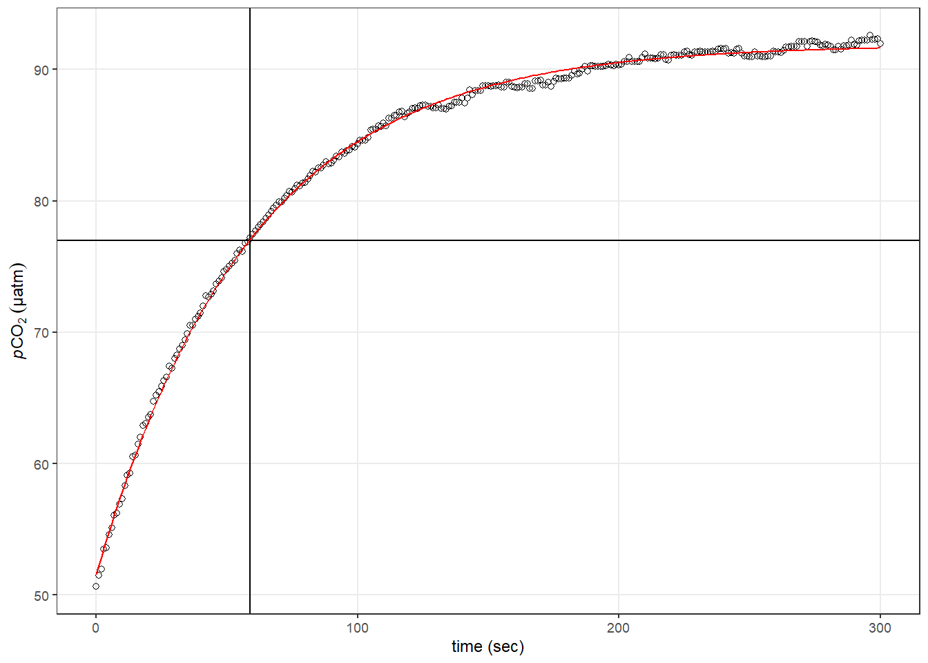

Example response time determination by non-linear least squares fit to the pCO₂ recovery signal after zeroing. The vertical line indicates the determined response time tau. The horizontal line indicates 63% of the difference between start and final fitted pCO₂.

ggsave(
  here::here(
    "output/Plots/Figures_publication/appendix",
    "Fig_A1.pdf"
  ),
  width = 83,
  height = 50,
  dpi = 300,
  units = "mm"
)

ggsave(
  here::here(
    "output/Plots/Figures_publication/appendix",
    "Fig_A1.png"
  ),
  width = 83,
  height = 50,
  dpi = 300,
  units = "mm"
)

rm(
  tm_flush_counter,
  fit,
  i_Zero_counter,
  tau,
  pCO2_corr_delta,
  pCO2_corr_end,
  pCO2_corr_start,
  resid_abs_mean
)

3.2.2 Flush intervals

Due to speculations about the dependence of determined response times (\(\tau\)) on the chosen duration of the fit interval, the response time \(\tau\) was determined for all zeroings and for folllowing duration limits:

150, 200, 250, 300, 350, 400, 450, 500 secs

3.2.3 Fitting algorithm

The code chunk below, fits the response to all Flush periods and duration limits, and creates a pdf with a plot for each individual fit.

pdf(
  file = here::here(
    "output/Plots/response_time",
    "tau_determination_pCO2_corr_flushperiods_nls.pdf"
  ),
  onefile = TRUE,
  width = 7,
  height = 4
)

for (i in unique(tm_flush$Zero_counter)) {
  for (max_duration in parameters$duration_intervals) {
    tm_flush_counter <- tm_flush %>%
      filter(Zero_counter == i, duration <= max_duration)
    
    fit <-
      try(tm_flush_counter %>%
            nls(pCO2_corr ~ SSasymp(duration, yf, y0, log_alpha), data = .),
          TRUE)
    
    if (class(fit) == "nls") {
      tau <- as.numeric(exp(-tidy(fit)[3, 2]))
      pCO2_corr_end <- as.numeric(tidy(fit)[1, 2])
      pCO2_corr_start <- as.numeric(tidy(fit)[2, 2])
      pCO2_corr_delta = pCO2_corr_end - pCO2_corr_start
      resid_abs_mean <- mean(abs(resid(fit)) / pCO2_corr_end) * 100
      
      temp <- as_tibble(
        bind_cols(
          Zero_counter = i,
          duration = max_duration,
          date_time = mean(tm_flush_counter$date_time),
          dep = mean(tm_flush_counter$dep),
          tem = mean(tm_flush_counter$tem),
          pCO2_corr = pCO2_corr_end,
          tau = tau,
          resid = resid_abs_mean
        )
      )
      
      if (exists("tau_values")) {
        tau_values <- bind_rows(tau_values, temp)
      }
      else {
        tau_values <- temp
      }
      
      if (resid_abs_mean > parameters$pCO2_resid_lim) {
        warn <- "orange"
      }
      else {
        warn <- "black"
      }
      
      print(
        augment(fit) %>%
          ggplot(aes(duration, pCO2_corr)) +
          geom_point(col = warn) +
          geom_line(aes(y = .fitted)) +
          geom_vline(xintercept = tau) +
          geom_hline(yintercept = pCO2_corr_start + 0.63 * (pCO2_corr_delta)) +
          labs(
            y = expression(italic(p)*CO[2] ~ (µatm)),
            x = "Duration of Flush period (s)",
            title = paste(
              "Zero_counter: ",
              i,
              "Tau: ",
              round(tau, 1),
              "Mean absolute residual (%): ",
              round(resid_abs_mean, 2)
            )
          ) +
          xlim(0, 600)
      )
      
    }
    
    
    else {
      temp <- as_tibble(
        bind_cols(
          Zero_counter = i,
          duration = max_duration,
          date_time = mean(tm_flush_counter$date_time),
          dep = mean(tm_flush_counter$dep),
          tem = mean(tm_flush_counter$tem),
          pCO2_corr = pCO2_corr_end,
          tau = NaN,
          resid = NaN
        )
      )
      
      if (exists("tau_values")) {
        tau_values <- bind_rows(tau_values, temp)
      }
      else {
        tau_values <- temp
      }
      
      print(
        tm_flush_counter %>%
          ggplot(aes(duration, pCO2_corr)) +
          geom_point(col = "red") +
          labs(
            y = expression(italic(p)*CO[2] ~ (µatm)),
            x = "Duration of Flush period (s)",
            title = paste("Zero_counter: ", i,
                          "nls model failed")
          ) +
          xlim(0, 600)
      )
      
    }
  }
}

dev.off()

rm(
  tm_flush_counter,
  fit,
  i,
  tau,
  pCO2_corr_delta,
  pCO2_corr_end,
  pCO2_corr_start,
  temp,
  max_duration,
  resid_abs_mean,
  warn
)

tau_values %>%
  write_csv(
    here::here(
      "data/intermediate/_merged_data_files/response_time",
      "tau_values.csv"
    )
  )

rm(tm_flush)

A pdf with plots of all individual response time fits can be accessed here.

In this pdf, response time fits that exceed the residual criterion (Mean absolute residual >1% of final pCO₂) are printed in orange. Data from flush periods without succesful fit are printed red.

3.2.4 Residual threshold

A mean absolute residual threshold of >1% of final pCO₂ was applied to all determined response times.

# define periods of different pumps used
max_Zero_counter <-
  max(unique(tau_values[tau_values$date_time < parameters$pump_switch, ]$Zero_counter))

tau_values <- tau_values %>%
  mutate(pump_power = if_else(Zero_counter <= max_Zero_counter, "1W", "8W"))


# subset determined tau values by residual threshold
tau_resid <- tau_values %>%
  group_by(Zero_counter) %>%
  mutate(resid_max = max(resid, na.rm = TRUE)) %>%
  filter(resid_max < parameters$pCO2_resid_lim) %>%
  select(-resid_max) %>%
  ungroup()

tau_resid_out <- tau_values %>%
  group_by(Zero_counter) %>%
  mutate(resid_max = max(resid, na.rm = TRUE)) %>%
  filter(resid_max > parameters$pCO2_resid_lim) %>%
  select(-resid_max) %>%
  ungroup()

# Flush periods where model failure occurred
tau_values %>%
  filter(is.na(resid)) %>%
  group_by(Zero_counter) %>%
  summarise(n()) %>%
  ungroup()

# Flush periods removed due to residual criterion
tau_resid_out %>%
  group_by(Zero_counter) %>%
  summarise(n()) %>%
  ungroup()

The first determined tau value, which is twice as high as the mean of all others for an unkown reason, was removed.

# mean tau of first RT determination
tau_resid %>%
  filter(Zero_counter == 2) %>%
  summarise(tau = mean(tau))

# mean tau of all RT determinations before pump switch, except first
tau_resid %>%
  filter(Zero_counter != 2, Zero_counter <= 20) %>%
  summarise(tau = mean(tau))

# remove first tau value which is twice as high as the mean of all others
tau_resid <- tau_resid %>%
  filter(Zero_counter != 2)

3.3 Analysis

3.3.1 General considerations

Estimated \(\tau\) values were only taken into account when stable environmental pCO₂ levels were present. Absence of stable environmental pCO₂ was assumed when the mean absolute fit residual was above 1 % of the final equilibrium pCO₂. If one model fit (irrespective the chosen fit interval length) of a particular flush period did not match that criterion, the flush period was ignored entirely. Usually, fits with higher duration did not meet this criterion. For some unexplained reason the first \(\tau\) determination resulted in values about twice as high as all other flush periods and was therefore removed as an outlier.

Metrics to characterize the fitting procedure include the number of:

n_Zero_counters <- tau_values %>%
  group_by(Zero_counter) %>%
  n_groups()

n_duration_intervals <-
  length(parameters$duration_intervals)

n_tau_max <- n_Zero_counters * length(parameters$duration_intervals)
n_tau_total <- nrow(tau_values %>% filter(!is.na(resid)))
n_tau_resid <- nrow(tau_resid)

• Flush periods: 76
• Duration intervals: 8
• Exercised response time fits: 608
• Succesful response times determinations: 576 (94.7)%
• \(\tau\)’s after removing groups of fits with high absolute fit residual: 416 (68.4 %)

It should be noted that all failed model fits occured in flush periods where the residual criterion was not meet by at least one other fit (i.e. fitting only failed under unstable conditions).

tau_values %>%
  ggplot(aes(resid)) +
  geom_histogram() +
  facet_wrap( ~ duration, labeller = label_both) +
  geom_vline(xintercept = parameters$pCO2_resid_lim) +
  labs(x = expression(Mean ~ absolute ~ residuals ~ ("%" ~ of ~ equilibrium ~
                                                       italic(p)*CO[2])))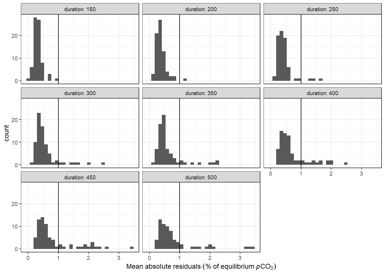

Histogram of residuals from fit displayed for the investigate durations of the fit interval. Vertical line represents the chosen threshold.

3.3.2 Fit interval length

No clear dependence of \(\tau\) on the length of the flushing period was found.

tau_resid %>%
  group_by(Zero_counter) %>%
  mutate(d_tau = tau - mean(tau)) %>%
  ggplot(aes(duration, d_tau)) +
  geom_hline(yintercept = 0) +
  geom_smooth() +
  geom_point() +
  facet_wrap( ~ Zero_counter, ncol = 4, labeller = label_both) +
  labs(x = "Duration (sec)", y = "Deviation from mean tau (sec)")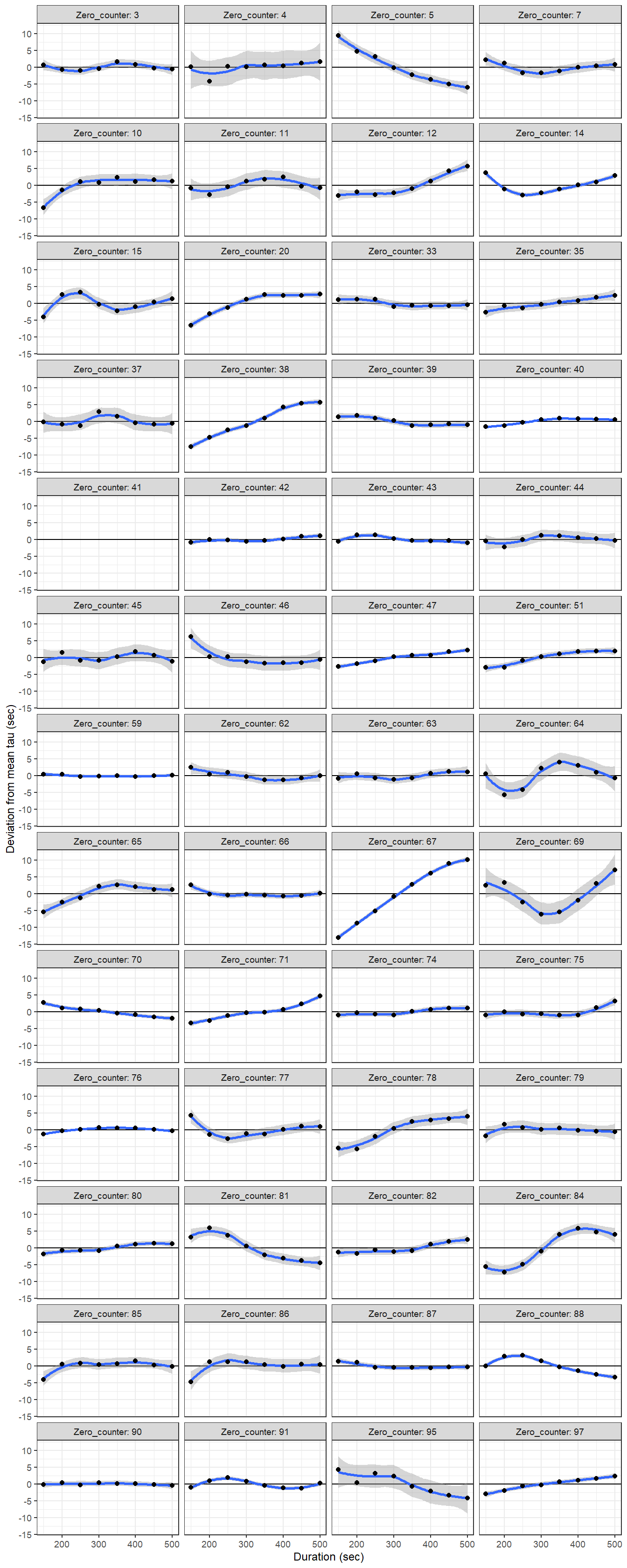

Determined tau values as a function of the fit interval duration, displayed individually for each flush period.

tau_resid %>%
  group_by(Zero_counter) %>%
  mutate(d_tau = tau - mean(tau)) %>%
  ggplot(aes(duration, d_tau, group = duration)) +
  geom_violin() +
  geom_point() +
  labs(x = "Duration (sec)", y = "Deviation from mean tau (sec)") +
  facet_wrap( ~ pump_power)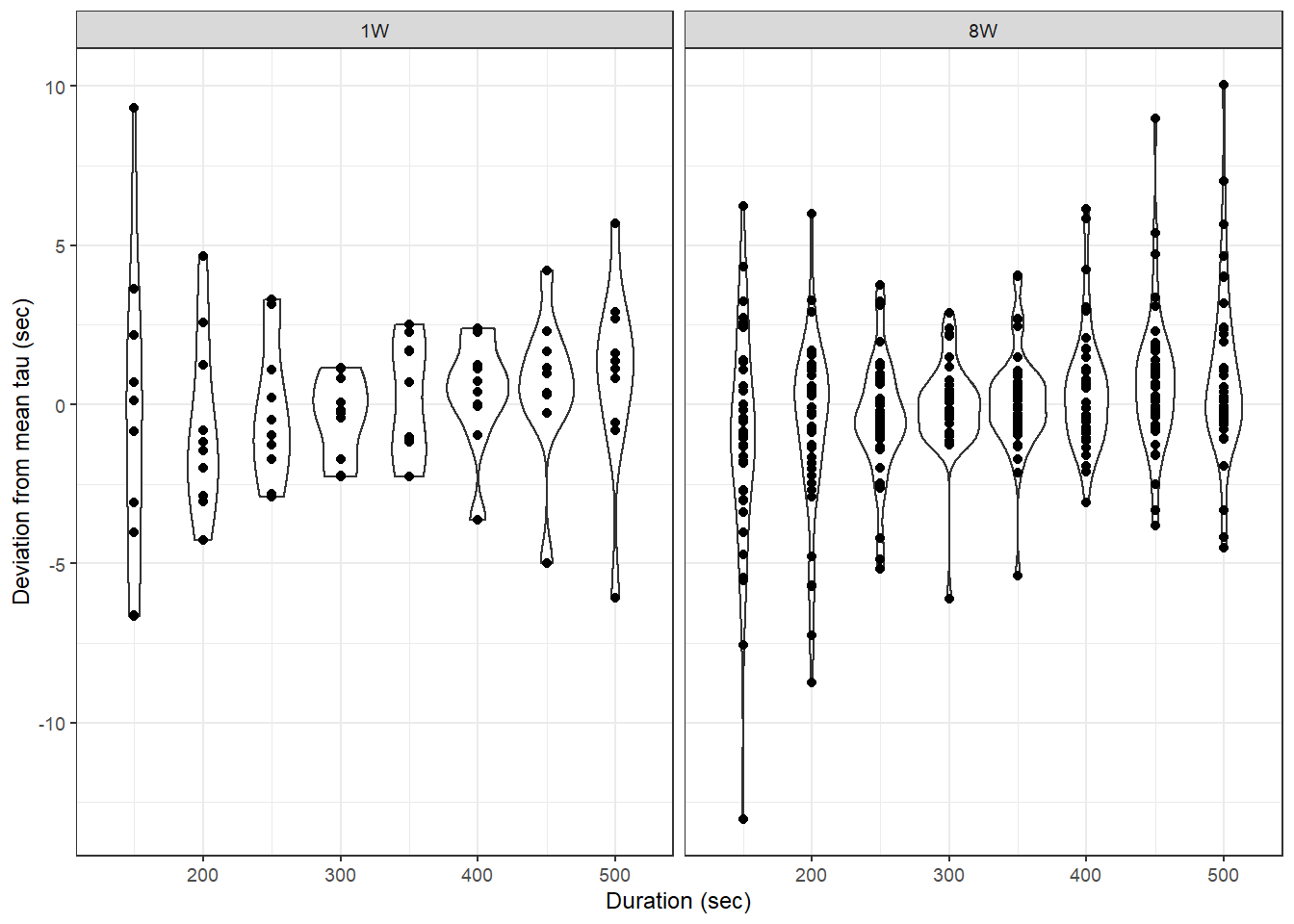

Determined tau values as a function of the fit interval duration, pooled for all flush period.

duration_min_tau_sd <- tau_resid %>%
  group_by(Zero_counter) %>%
  mutate(d_tau = tau - mean(tau)) %>%
  ungroup() %>%
  group_by(duration) %>%
  summarise(d_tau_sd = sd(d_tau, na.rm = TRUE)) %>%
  ungroup() %>%
  slice(which.min(d_tau_sd)) %>%
  select(duration) %>%
  pull()

The lowest standard deviation of \(\tau\) values was found for a duration of:

• 300 sec

\(\tau\) values determined with this duration were filtered for further analysis.

tau_resid <- tau_resid %>%
  filter(duration == duration_min_tau_sd) %>%
  select(-duration)

rm(duration_min_tau_sd) 

3.3.3 Time series of \(\tau\)

No obvious change of \(\tau\) over time was detected, but a dependence on the pump used.

ggplot() +
  geom_smooth(
    data = tau_resid %>% filter(dep < 10),
    aes(date_time, tau, linetype = pump_power),
    method = "lm",
    se = FALSE,
    col = "red"
  ) +
  geom_point(data = tau_resid,
             aes(date_time, tau, col = dep, shape = pump_power)) +
  scale_color_viridis_c(name = "Depth (m)") +
  labs(y = "Tau (sec)", x = "Date") +
  ylim(0, NA)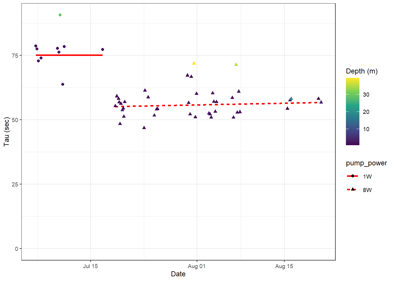

Tau for all Zeroings with color representing water depth. Red lines represent linear regression trends for tau determined in surface waters (<10m).

3.3.4 Temperature dependence

A temperature dependence of determined response times \(\tau\) was found, with similar slopes but different intercepts for both pumps used.

tau_resid %>%
  ggplot(aes(tem, tau, col = dep)) +
  geom_smooth(method = "lm") +
  geom_point() +
  scale_color_viridis_c(name = "Depth (m)") +
  labs(y = "Tau (sec)", x = "Temperature (deg C)") +
  facet_wrap( ~ pump_power, labeller = label_both)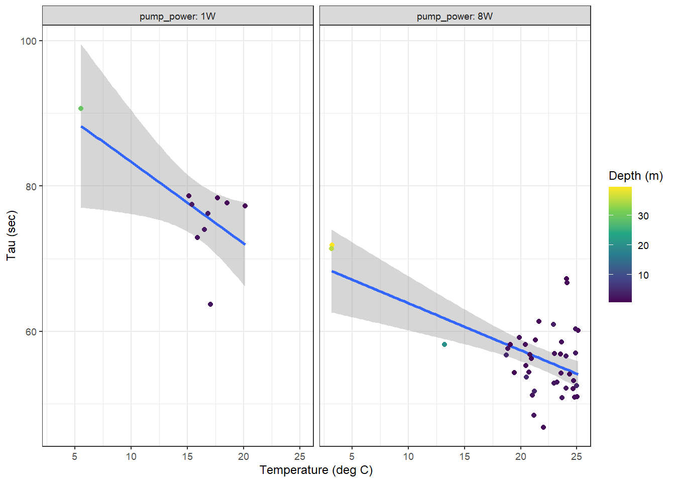

Tau as a function of temperature for all zeroings determined with low power (left) and strong (right) pump. Color represents the water depth.

For the response times determined near the surface (<10m, restricted temperature range), no clear temperature dependence of \(\tau\) was detected.

tau_resid %>%
  filter(dep < 10) %>%
  ggplot(aes(tem, tau, col = dep)) +
  geom_smooth(method = "lm") +
  geom_point() +
  scale_color_viridis_c(name = "Depth (m)") +
  labs(y = "Tau (sec)", x = "Temperature (deg C)") +
  facet_wrap( ~ pump_power, labeller = label_both)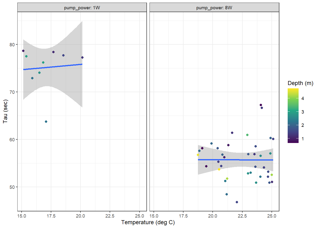

Surface tau (<10m) as a function of temperature for all zeroings determined with low power (left) and strong (right) pump. Color represents the water depth.

3.3.5 Final \(\tau\) values

The mean \(\tau\) values are:

# calculate mean tau for each pump
tau_mean <- tau_resid %>% 
  group_by(pump_power) %>% 
  summarise(tau = mean(tau, na.rm = TRUE))

tau_mean

# A tibble: 2 x 2
  pump_power   tau
  <chr>      <dbl>
1 1W          76.7
2 8W          56.5

The linear response of \(\tau\) on water temperature was fitted as:

# fit linear regression of tau for each pump
tau_fit <- tau_resid %>%
  nest_by(pump_power) %>%
  mutate(fit = list(lm(tau ~ tem, data = data))) %>%
  summarise(tidy(fit)) %>%
  select(pump_power, term, estimate) %>%
  spread(term, estimate)

tau_fit

# A tibble: 2 x 3
# Groups:   pump_power [2]
  pump_power `(Intercept)`    tem
  <chr>              <dbl>  <dbl>
1 1W                  94.5 -1.12 
2 8W                  70.4 -0.648

tau_fit %>% write_csv(here::here(
  "data/intermediate/_merged_data_files/response_time",
  "tau_fit.csv"
))

# clean workspace
rm(list = setdiff(ls(), c(
  "tau_resid", "tau_fit", "parameters"
)))

Only the T-dependent \(\tau\) estimate will be applied to correct the recorded pCO₂ profiles.

4 Response time correction

4.1 Data preparation

Following tasks were performed to prepare data for the response time correction:

• Select only profiles
• Assign deployment periods with 1W- and 8W- pump

tm <- read_csv(here::here("data/intermediate/_merged_data_files/merging_interpolation",
                          "tm.csv"),
               col_types = cols(ID = col_character(),
                                pCO2_analog = col_double(),
                                pCO2_corr = col_double(),
                                Zero = col_factor(),
                                Flush = col_factor(),
                                Zero_counter = col_integer(),
                                deployment = col_integer(),
                                duration = col_double(),
                                mixing = col_character(),
                                lat = col_double(),
                                lon = col_double()))

# select relevant columns
tm <- tm %>%
  select(date_time, ID, type, station, dep, sal, tem,
         Zero, Flush, pCO2_corr, deployment, Zero_counter)

# filter profiles
tm <- tm %>% 
  filter(type == "P")

# assign pump types
tm <- tm %>%
  group_by(ID, station) %>% 
  mutate(duration = as.numeric(date_time - min(date_time)),
         pump_power = if_else(date_time < parameters$pump_switch, "1W", "8W")) %>%
  arrange(date_time)

• Include manually derived meta-information about the profiling status. Those meta data were assigned through visual inspection of each profiles (depth vs time) and distinguish phases of the casts, in particular the continuous up and downcast operation.

# Load profile meta data 
meta <- read_csv(here::here("data/input/TinaV/Sensor",
                            "Sensor_meta.csv"),
                 col_types = cols(ID = col_character()))


# Merge profiles and meta information 
tm <- full_join(tm, meta)
rm(meta)


# assign profiling phases according to meta data

tm <- tm %>% 
  mutate(phase = "standby",
         phase = if_else(duration >= start &
                           duration < down & 
                           !is.na(down) &
                           !is.na(start),
                         "down", phase),
         phase = if_else(duration >= down  & 
                           duration < lift & 
                           !is.na(lift) & 
                           !is.na(down ),   
                         "low",  phase),
         phase = if_else(duration >= lift  & 
                           duration < up   & 
                           !is.na(up  ) & 
                           !is.na(lift  ),  
                         "mid",  phase),
         phase = if_else(duration >= up    & 
                           duration < end  & 
                           !is.na(end ) & 
                           !is.na(up   ),   
                         "up",   phase))

tm <- tm %>% 
  select(-c(start, down, lift, up, end, comment))

# discard zero and flush periods
tm <- tm %>% 
  filter(Zero == 0, Flush == 0)

• Subset reference pCO₂ recordings at the end of equilibration periods executed at constant depth

tm_pCO2_equi <- tm %>% 
  filter(phase %in% c("mid")) %>% 
  group_by(ID, station) %>% 
  top_n(5, row_number()) %>% 
  summarise(date_time = mean(date_time),
            duration = mean(duration),
            pCO2_corr = mean(pCO2_corr, na.rm = TRUE),
            dep = mean(dep, na.rm = TRUE)) %>% 
  ungroup()


# tm_pCO2_equi %>% 
#  write_csv(here::here("data/intermediate/_merged_data_files/response_time",
#                       "tm_pCO2_equi.csv"))

cast_dep <- tm %>%
  pivot_longer(c(dep, pCO2_corr), names_to = "parameter", values_to = "value")

cast_dep_equi <- tm_pCO2_equi %>%
  pivot_longer(c(dep, pCO2_corr), names_to = "parameter", values_to = "value")

max_duration <- round(max(cast_dep$duration) / 1000, 0) * 1000

cast_dep_equi_sub <- cast_dep_equi %>%
  filter(ID == parameters$example_ID,
         station == parameters$example_station)


cast_dep %>%
  filter(ID == parameters$example_ID,
         station == parameters$example_station) %>%
  ggplot(aes(duration, value, col = phase)) +
  geom_point(size = 0.5) +
  geom_point(data = cast_dep_equi_sub, aes(duration, value), col = "black") +
  scale_y_reverse() +
  scale_x_continuous(breaks = seq(0, 6000, 500)) +
  labs(title = str_c(
    "Date: ",
    parameters$example_ID,
    " | Station: ",
    parameters$example_station
  )) +
  facet_grid(parameter ~ ., scales = "free_y")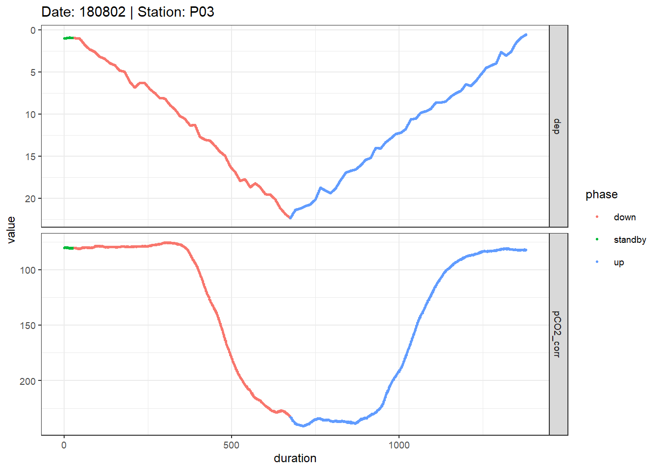

Example timeseries of profiling depth and pCO₂. Colors represent manually assigned profiling phases. The black points represent reference data collected at the end of the mid equilibration period.

rm(cast_dep, cast_dep_equi, cast_dep_equi_sub, max_duration)

cast_dep <- tm %>% 
  pivot_longer(c(dep, pCO2_corr), names_to = "parameter", values_to = "value")

cast_dep_equi <- tm_pCO2_equi %>% 
  pivot_longer(c(dep, pCO2_corr), names_to = "parameter", values_to = "value")

max_duration <- round(max(cast_dep$duration)/1000,0)*1000

pdf(file=here::here("output/Plots/response_time",
                    "time_series_depth_pCO2_corr_by_profile.pdf"),
    onefile = TRUE, width = 7, height = 4)

for(i_ID in unique(cast_dep$ID)){
  for(i_station in unique(cast_dep$station)){

    if (nrow(cast_dep %>% filter(ID == i_ID, station == i_station)) > 0){
      
        cast_dep_equi_sub <- cast_dep_equi %>%
        filter(ID == i_ID,
               station == i_station)

      print(
      
        cast_dep %>%
        filter(ID == i_ID,
               station == i_station) %>%
        ggplot(aes(duration, value, col=phase))+
        geom_point(size=0.5)+
        geom_point(data = cast_dep_equi_sub, aes(duration, value), col="black")+
        scale_y_reverse()+
        scale_x_continuous(breaks = seq(0,6000,500))+
        labs(title = str_c("Date: ",i_ID," | Station: ",i_station))+
        facet_grid(parameter~., scales = "free_y")+
        theme_bw()
      
      )

    }

  }
}

dev.off()

rm(cast_dep, cast_dep_equi, cast_dep_equi_sub, i_station, i_ID, max_duration)

A pdf with all timeseries plots of profiling depth and pCO₂ can be accessed here.

4.1.1 Profiling speed

We plotted a histogram of mean downcast profiling speed (m/s) per profile and calculated the mean profiling speed.

downcast <- tm %>%
  filter(phase == "down")

downcast_speed <- downcast %>%
  group_by(ID, station) %>%
  summarise(
    duration = as.numeric(max(date_time) - min(date_time)),
    distance = max(dep) - min(dep),
    speed = distance / duration
  ) %>%
  ungroup()

downcast_speed %>% 
  ggplot(aes(speed)) +
  geom_histogram()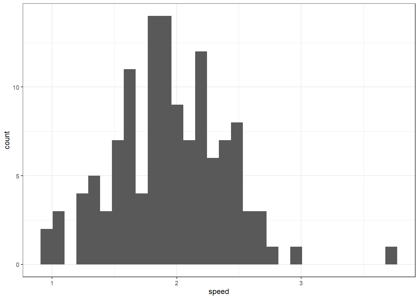

downcast_speed %>% 
  summarise(mean(speed),
            sd(speed))

# A tibble: 1 x 2
  `mean(speed)` `sd(speed)`
          <dbl>       <dbl>
1          1.95       0.448

rm(downcast, downcast_speed)

4.2 Apply correction

The executed response time correction featured the following aspects:

• Correction according to Fiedler et al. (2013)
• RT: T-dependent response times applied
• tau_factor: Factors of 0.8, 1, 1.2, 1.4, 1.6 were applied to determined tau values
• Post-smoothing: 30 sec running mean (eg across 15 observations at 2 sec measurement frequency)

# Define function for response time correction after Bittig et al, 2018

# RT_corr_Bit <- function(c1, c0, dt, tau) {
#   (1 / (2 * ((1 + (
#     2 * tau / dt
#   )) ^ (-1)))) * (c1 - (1 - (2 * ((
#     1 + (2 * tau / dt)
#   ) ^ (
#     -1
#   )))) * c0)
# }

# Define function for response time correction after Fiedler et al, 2013

RT_corr <- function(c1, c0, dt, tau) {
(c1 - (c0 * exp(-dt/tau)) ) /
    (1 - exp(-dt/tau))
}


# Assign T-dependent response time (tau) values

tau_fit <- tau_fit %>%
  rename(tau_intercept = `(Intercept)`, tau_slope = tem)

tm <- full_join(tm, tau_fit)

tm <- tm %>%
  mutate(tau = tau_intercept + tau_slope * tem) %>%
  select(-tau_intercept,-tau_slope)


# Prepare data set for RT correction

tm <- tm %>%
  arrange(date_time) %>%
  mutate(dt = as.numeric(as.character(date_time - lag(date_time))))


# determine measurement frequency of sensor

freq <- tm %>%
  filter(dt < 13) %>%
  group_by(ID) %>%
  summarise(dt_mean = round(mean(dt, na.rm = TRUE), 0))

tm <- full_join(tm, freq)

# apply tau factors

tm <- expand_grid(tm, tau_factor = parameters$tau_factors)

tm <- tm %>%
  mutate(tau_test = tau * tau_factor)


# Apply RT correction to profiling data

for (i_ID in unique(tm$ID)) {

  freq_sub <- freq %>% filter(ID == i_ID) %>% pull(dt_mean)
  
  # window width for smoothing
  window <- parameters$smoothing_duration / freq_sub
  # function for rolling mean
  rolling_mean   <-
    rollify( ~ mean(.x, na.rm = TRUE), window = window)
  
  # data subset for each cruise day, and RT correction per station
  tm_sub <- tm %>%
    filter(ID == i_ID) %>%
    group_by(station, tau_factor) %>%
    mutate(
      pCO2_RT = RT_corr(pCO2_corr, lag(pCO2_corr), dt, tau_test),
      pCO2_RT = if_else(pCO2_RT %in% c(Inf,-Inf), NaN, pCO2_RT),
      # pCO2_RT_Bit = RT_corr_Bit(pCO2_corr, lag(pCO2_corr), dt, tau_test),
      # pCO2_RT_Bit = if_else(pCO2_RT_Bit %in% c(Inf,-Inf), NaN, pCO2_RT_Bit),
      window = window,
      pCO2 = rolling_mean(pCO2_RT)
      # pCO2_Bit = rolling_mean(pCO2_RT_Bit)
    ) %>%
    ungroup()
  
  # time shift RT corrected data
  shift <- as.integer(as.character(window / 2))
  
  tm_sub <- tm_sub %>%
    group_by(station, tau_factor) %>%
    mutate(pCO2 = lead(pCO2, shift)) %>%
    ungroup()
  
  # append to new data frame
  if (exists("tm_RT")) {
    tm_RT <- bind_rows(tm_RT, tm_sub)
  }
  else{
    tm_RT <- tm_sub
  }
  
  rm(tm_sub, freq_sub, rolling_mean, shift, window)
  
}

tm <- tm_RT

rm(i_ID, freq, RT_corr, tau_fit, tau_resid, tm_RT)

5 Diagnosis

tm %>% 
  ggplot(aes(pCO2_RT - pCO2_RT_Bit)) +
  geom_histogram(binwidth = 5) +
  scale_y_log10() +
  scale_x_continuous(limits = c(-20,20))

min(tm$pCO2_RT - tm$pCO2_RT_Bit, na.rm = TRUE)
max(tm$pCO2_RT - tm$pCO2_RT_Bit, na.rm = TRUE)

In the following, the success of the response time correction is assessed through the

• visual inspection of RT corrected profiles,

as well as the offset between the downcast and:

• Upcast
• pCO₂ reference value (recorded after equilibration period during upcast)

The offset comparison requires to discretize the continous depth recording. Depth intervals of 1m were chosen.

First, we analyze all profiles individually. Later we’ll merge the information across profiles and come up with a single metric to quantify the quality of the response time correction

5.1 Individual profiles

equi_cast <- tm_pCO2_equi %>%
  filter(ID == parameters$example_ID,
         station == parameters$example_station)

tm %>%
  filter(
    ID == parameters$example_ID,
    station == parameters$example_station,
    phase %in% c("up", "down")
  ) %>%
  ggplot() +
  geom_path(aes(pCO2_corr, dep, linetype = phase, col = "raw")) +
  geom_path(aes(pCO2, dep, linetype = phase, col = "corrected")) +
  geom_point(data = equi_cast, aes(pCO2_corr, dep)) +
  scale_y_reverse() +
  coord_cartesian(ylim = c(35, 0),
                  xlim = c(70, 270)) +
  scale_color_brewer(palette = "Set1", name = "") +
  labs(title = str_c(
    "Date: ",
    parameters$example_ID,
    " | Station: ",
    parameters$example_station
  )) +
  facet_grid(tau_factor ~ ., labeller = label_both)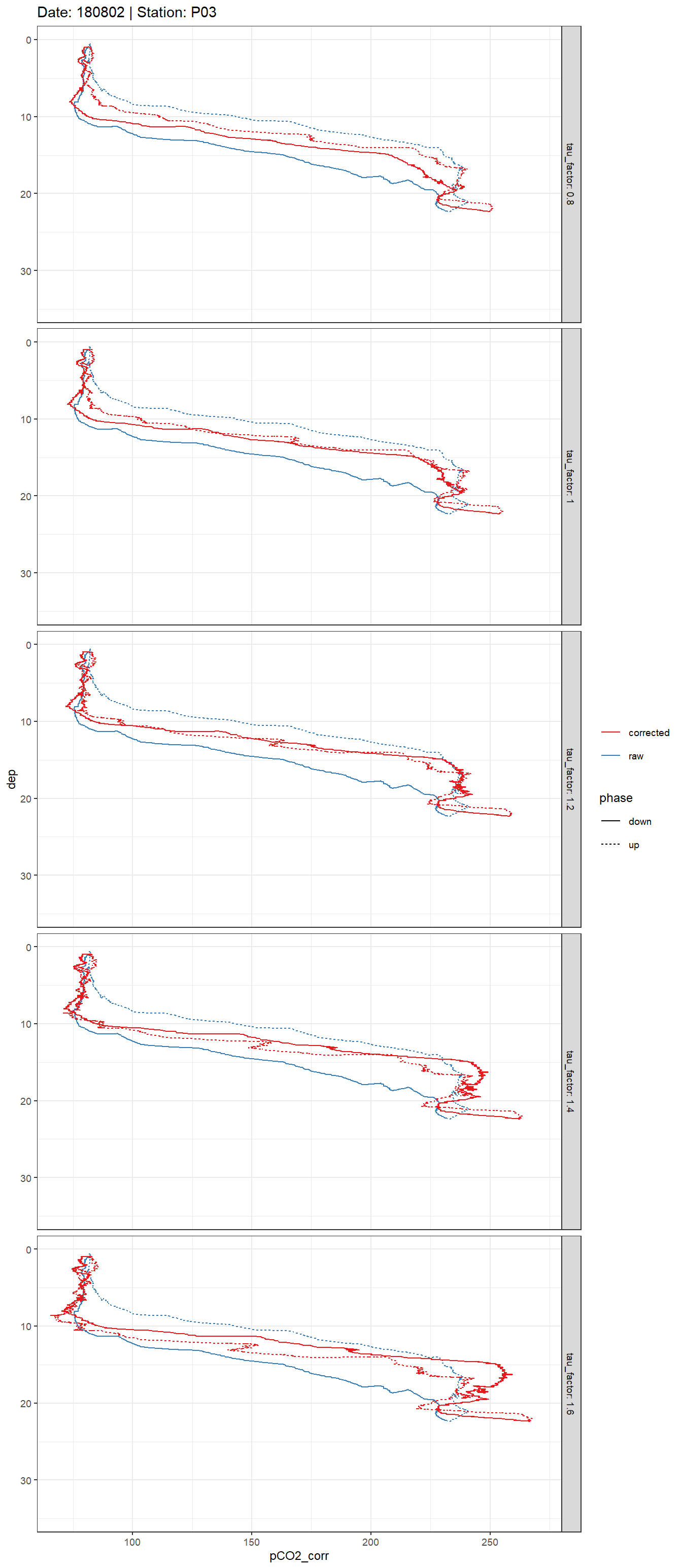

Example plot of response time corrected and raw pCO₂ profiles. Panels highlight the effect of constant vs T-dependent tau estimates (columns) and the optimization by applying a constant factor (rows).

rm(equi_cast)

A pdf with all timeseries plots of profiling depth and pCO₂ can be accessed here

pdf(
  file = here::here("output/Plots/response_time",
                    "profiles_pCO2.pdf"),
  onefile = TRUE,
  width = 7,
  height = 11
)

for (i_ID in unique(tm$ID)) {
  for (i_station in unique(tm$station)) {
    if (nrow(tm %>% filter(ID == i_ID, station == i_station)) > 0) {
      equi_cast <- tm_pCO2_equi %>%
        filter(ID == i_ID,
               station == i_station)
      
      print(
        tm %>%
          filter(ID == i_ID,
                 station == i_station,
                 phase %in% c("up", "down")) %>%
          ggplot() +
          geom_path(aes(
            pCO2_corr, dep, linetype = phase, col = "raw"
          )) +
          geom_path(aes(
            pCO2, dep, linetype = phase, col = "corrected"
          )) +
          geom_point(data = equi_cast, aes(pCO2_corr, dep)) +
          scale_y_reverse() +
          coord_cartesian(ylim = c(35, 0),
                          xlim = c(70, 270)) +
          scale_color_brewer(palette = "Set1", name = "") +
          labs(title = str_c(
            "Date: ", i_ID, " | Station: ", i_station
          )) +
          theme_bw() +
          facet_grid(tau_factor ~ ., labeller = label_both)
        
      )
      
      
    }
    
  }
}

dev.off()

rm(equi_cast, i_ID, i_station)

5.2 Down- vs upcast

# pCO2 offset up - down cast
tm_grid <- tm %>%
  filter(phase %in% c("down", "up")) %>%
  mutate(dep_grid = as.numeric(as.character(cut(
    dep, seq(0, 40, 1), seq(0.5, 39.5, 1)
  ))),
  tau_factor = as.factor(tau_factor)) %>%
  select(ID, station, tau_factor, p_type, dep_grid, phase, pCO2_corr, pCO2) %>%
  group_by(ID, station, tau_factor, p_type, dep_grid, phase) %>%
  summarise_all("mean", na.rm = TRUE) %>%
  ungroup() %>%
  pivot_longer(cols = c(pCO2_corr, pCO2), names_to = "correction") %>%
  pivot_wider(names_from = phase, values_from = value) %>%
  mutate(
    pCO2_delta = up - down,
    pCO2_up_down_average = (down + up) / 2,
    pCO2_delta_rel = 100 * pCO2_delta / pCO2_up_down_average
  )

tm_pCO2_equi_grid <- tm_pCO2_equi %>%
  mutate(dep_grid = as.numeric(as.character(cut(
    dep, seq(0, 40, 1), seq(0.5, 39.5, 1)
  )))) %>%
  select(ID, station, dep_grid, pCO2_equi = pCO2_corr)

tm_pCO2_equi_grid_sub <- tm_pCO2_equi_grid %>%
  filter(ID == parameters$example_ID,
         station == parameters$example_station)


tm_grid %>%
  filter(ID == parameters$example_ID,
         station == parameters$example_station) %>%
  arrange(dep_grid) %>%
  ggplot() +
  geom_path(aes(down, dep_grid, col = correction, linetype = "down")) +
  geom_path(aes(up, dep_grid, col = correction, linetype = "up")) +
  geom_point(data = tm_pCO2_equi_grid_sub, aes(pCO2_equi, dep_grid)) +
  scale_y_reverse() +
  coord_cartesian(ylim = c(35, 0),
                  xlim = c(70, 270)) +
  scale_linetype(name = "cast") +
  scale_color_brewer(palette = "Set1", direction = -1) +
  labs(
    y = "Depth [m]",
    x = expression(italic(p) * CO[2] ~ (µatm)),
    title = str_c(
      "Date: ",
      parameters$example_ID,
      " | Station: ",
      parameters$example_ID
    )
  ) +
  facet_grid(tau_factor ~ ., labeller = label_both)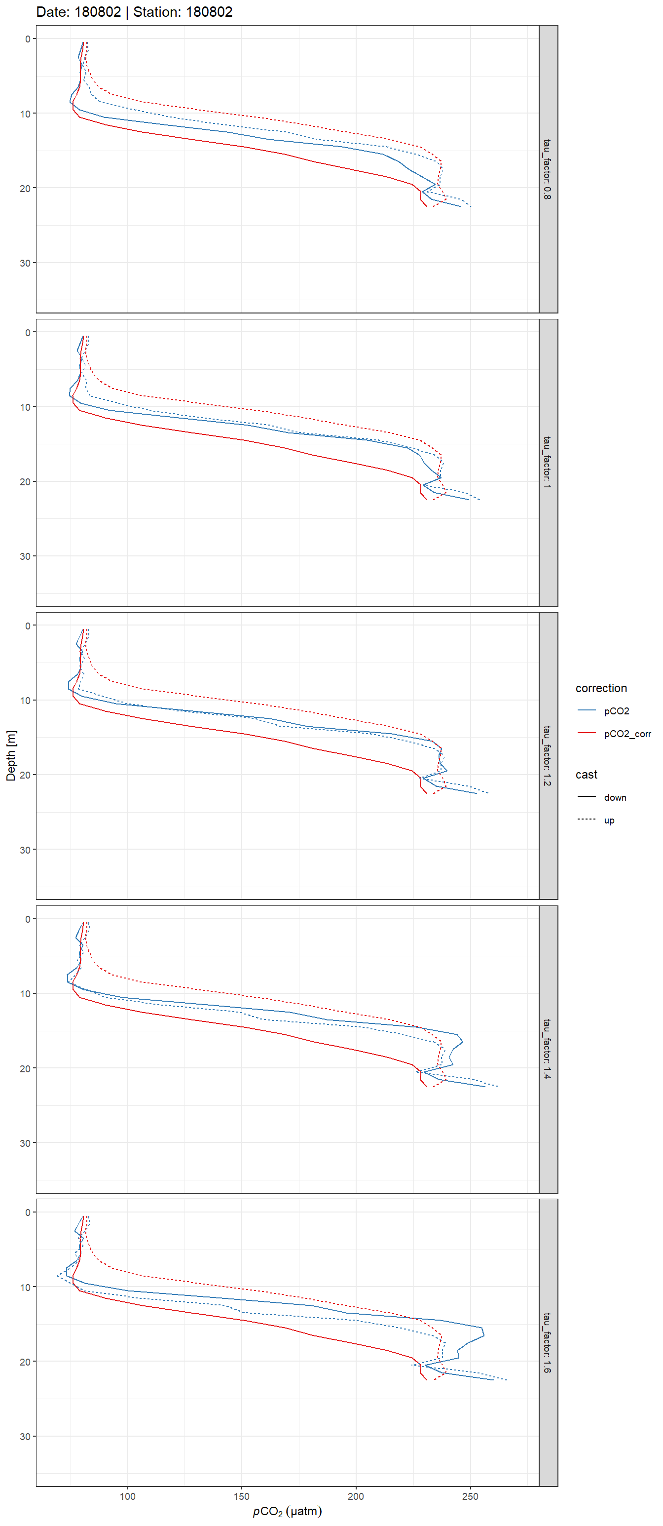

Example plot of discretized, response time corrected and raw pCO₂ profiles. Panels highlight the effect of constant vs T-dependent tau estimates (columns) and the optimization by applying a constant factor (rows). The black point indicates the reference pCO₂ value.

rm(tm_pCO2_equi_grid_sub)

A pdf with all discretized pCO₂ profiles can be assessed here

pdf(
  file = here::here("output/Plots/response_time",
                    "profiles_pCO2_grid.pdf"),
  onefile = TRUE,
  width = 7,
  height = 11
)

for (i_ID in unique(tm_grid$ID)) {
  for (i_station in unique(tm_grid$station)) {
    if (nrow(tm_grid %>% filter(ID == i_ID, station == i_station)) > 0) {
      tm_pCO2_equi_grid_sub <- tm_pCO2_equi_grid %>%
        filter(ID == i_ID,
               station == i_station)
      
      print(
        tm_grid %>%
          filter(ID == i_ID,
                 station == i_station) %>%
          arrange(dep_grid) %>%
          ggplot() +
          geom_path(aes(
            down, dep_grid, col = correction, linetype = "down"
          )) +
          geom_path(aes(
            up, dep_grid, col = correction, linetype = "up"
          )) +
          geom_point(data = tm_pCO2_equi_grid_sub, aes(pCO2_equi, dep_grid)) +
          scale_y_reverse() +
          coord_cartesian(ylim = c(35, 0),
                          xlim = c(70, 270)) +
          scale_linetype(name = "cast") +
          scale_color_brewer(palette = "Set1", direction = -1) +
          labs(
            y = "Depth [m]",
            title = str_c("Date: ", i_ID, " | Station: ", i_station)
          ) +
          theme_bw() +
          facet_grid(tau_factor ~ ., labeller = label_both)
        
      )
      
      rm(tm_pCO2_equi_grid_sub)
    }
    
  }
}

dev.off()

tm_grid %>%
  filter(
    ID == parameters$example_ID,
    station == parameters$example_station,
    correction == "pCO2"
  ) %>%
  arrange(dep_grid) %>%
  ggplot(aes(pCO2_delta, dep_grid, col = as.factor(tau_factor))) +
  geom_path() +
  geom_point() +
  scale_y_reverse(breaks = seq(0, 40, 2)) +
  scale_color_discrete(name = "tau factor") +
  labs(
    x = expression(Delta ~ italic(p) * CO[2] ~ (µatm)),
    y = "Depth [m]",
    title = str_c(
      "Date: ",
      parameters$example_ID,
      " | Station: ",
      parameters$example_station
    )
  ) +
  geom_vline(xintercept = 0) +
  geom_vline(xintercept = c(-10, 10), col = "red")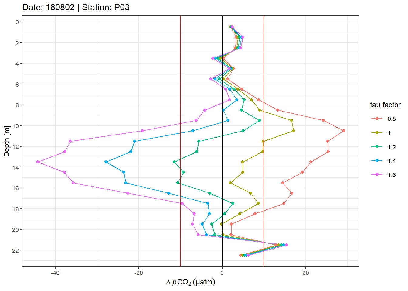

Example plot of absolute pCO₂ offset profiles. Panels highlight the effect of constant vs T-dependent tau estimates. Colour indicates the optimization by applying a constant factor to tau. Vertical red lines mark an arbitray 10 µatm pCO₂ threshold.

pdf(
  file = here::here(
    "output/Plots/response_time",
    "profiles_pCO2_delta_grid.pdf"
  ),
  onefile = TRUE,
  width = 7,
  height = 7
)

for (i_ID in unique(tm_grid$ID)) {
  for (i_station in unique(tm_grid$station)) {
    if (nrow(tm_grid %>% filter(ID == i_ID, station == i_station)) > 0) {
      print(
        tm_grid %>%
          filter(ID == i_ID,
                 station == i_station,
                 correction == "pCO2") %>%
          arrange(dep_grid) %>%
          ggplot(aes(
            pCO2_delta, dep_grid, col = as.factor(tau_factor)
          )) +
          geom_path() +
          geom_point() +
          scale_y_reverse(breaks = seq(0, 40, 2)) +
          scale_color_discrete(name = "tau factor") +
          labs(
            x = "delta pCO2 [µatm]",
            y = "Depth [m]",
            title = str_c("Date: ", i_ID, " | Station: ", i_station)
          ) +
          geom_vline(xintercept = 0) +
          geom_vline(xintercept = c(-10, 10), col = "red") +
          theme_bw()
        
      )
      
    }
    
  }
}

dev.off()

A pdf with all absolute pCO₂ offset profiles can be assessed here.

tm_grid %>%
  filter(
    ID == parameters$example_ID,
    station == parameters$example_station,
    correction == "pCO2"
  ) %>%
  arrange(dep_grid) %>%
  ggplot(aes(pCO2_delta_rel, dep_grid, col = as.factor(tau_factor))) +
  geom_path() +
  geom_point() +
  scale_y_reverse(breaks = seq(0, 40, 2)) +
  scale_color_discrete(name = "tau factor") +
  labs(
    x = expression(Delta ~ italic(p) * CO[2] ~ ("%" ~ of ~ absolute ~ value)),
    y = "Depth [m]",
    title = str_c(
      "Date: ",
      parameters$example_ID,
      " | Station: ",
      parameters$example_station
    )
  ) +
  geom_vline(xintercept = 0) +
  geom_vline(xintercept = c(-10, 10), col = "red")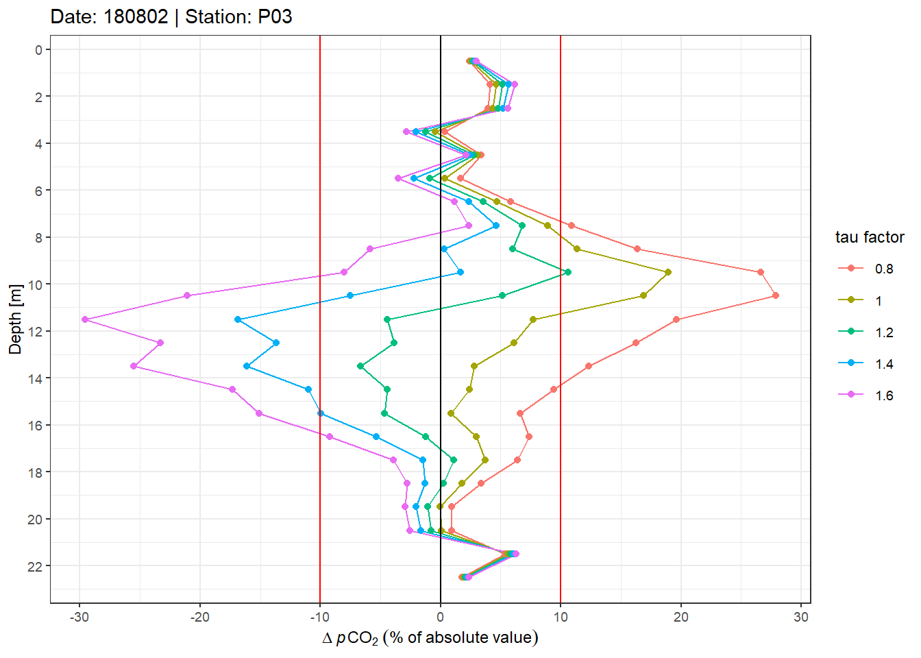

Example plot of relative offset pCO₂ profiles. Panels highlight the effect of constant vs T-dependent tau estimates. Colour indicates the optimization by applying a constant factor to tau. Vertical red lines mark an arbitray 10% threshold.

A pdf with all relative pCO₂ offset profiles can be assessed here.

pdf(
  file = here::here(
    "output/Plots/response_time",
    "profiles_pCO2_delta_rel_grid.pdf"
  ),
  onefile = TRUE,
  width = 7,
  height = 7
)

for (i_ID in unique(tm_grid$ID)) {
  for (i_station in unique(tm_grid$station)) {
    if (nrow(tm_grid %>% filter(ID == i_ID, station == i_station)) > 0) {
      print(
        tm_grid %>%
          filter(ID == i_ID,
                 station == i_station,
                 correction == "pCO2") %>%
          arrange(dep_grid) %>%
          ggplot(aes(
            pCO2_delta_rel, dep_grid, col = as.factor(tau_factor)
          )) +
          geom_path() +
          geom_point() +
          scale_y_reverse(breaks = seq(0, 40, 2)) +
          scale_color_discrete(name = "tau factor") +
          labs(
            x = "delta pCO2 [% of absolute value]",
            y = "Depth [m]",
            title = str_c("Date: ", i_ID, " | Station: ", i_station)
          ) +
          geom_vline(xintercept = 0) +
          geom_vline(xintercept = c(-10, 10), col = "red") +
          theme_bw()
        
      )
      
    }
    
  }
}

dev.off()

5.3 Downcast vs reference value

Referenced values were obtained occasionally through interuption of the profiling measurements to achieve sensor equilibration. Readings under equilibrated conditions were extracted and compared to the corresponding continous cast value.

tm_equi_delta <- full_join(tm_grid, tm_pCO2_equi_grid) %>% 
  filter(!is.na(pCO2_equi)) %>% 
  mutate(pCO2_delta_equi = down - pCO2_equi,
         pCO2_delta_equi_rel = 100 * pCO2_delta_equi / pCO2_equi)

tm_equi_delta %>%
  filter(tau_factor == parameters$tau_factor_used, correction == "pCO2") %>%
  ggplot(aes(pCO2_equi, pCO2_delta_equi)) +
  geom_hline(yintercept = 0) +
  geom_point() +
  labs(x = expression(Reference ~ italic(p)*CO[2] ~ (µatm)),
       y = expression(Delta ~ italic(p)*CO[2] ~ from ~ reference ~ (µatm)))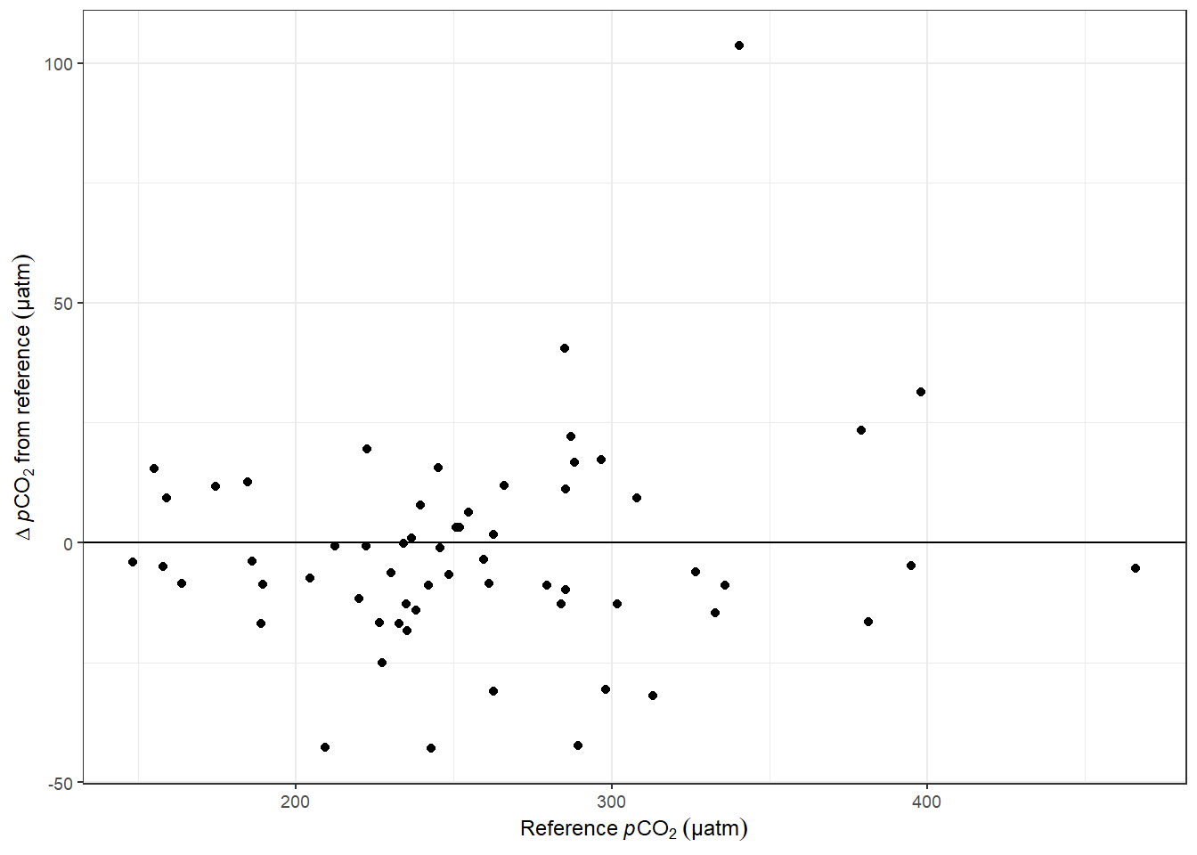

Offset between pCO₂ downcast and upcast reference value as a function of absolute pCO₂.

tm_equi_delta %>%
  ggplot(aes(as.factor(tau_factor), pCO2_delta_equi, fill = correction)) +
  geom_hline(yintercept = 0) +
  geom_violin() +
  scale_fill_brewer(palette = "Set1")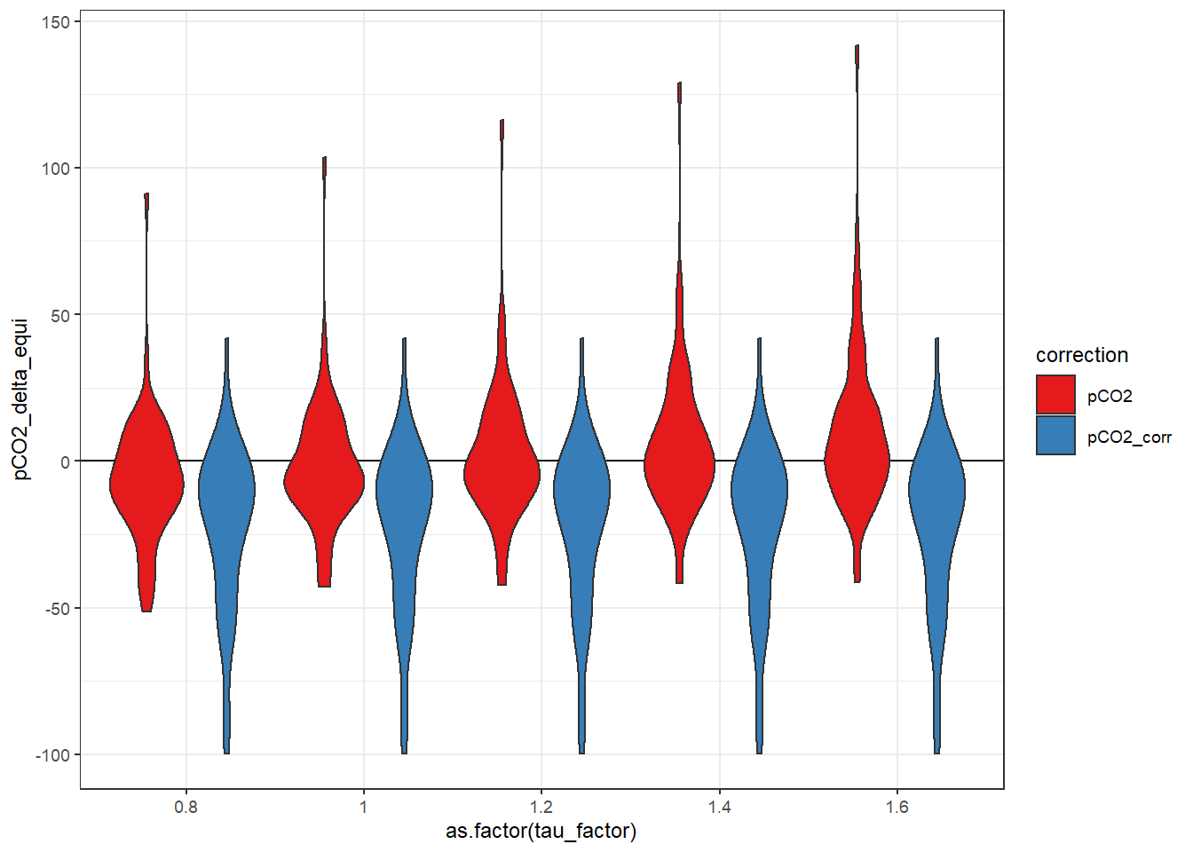

Offset between pCO₂ downcast and upcast reference value. Panels highlight the effect of constant vs T-dependent tau estimates. Colour distinguish raw and corrected offsets.

5.4 Summary metrics

In order to decide, which conditions resulted in the best response correction the mean absoulte and relative pCO₂ offset across all profiles was calculated for:

• the offset between downcast and reference value
• the offset between downcast and upcast
• T-dependent tau
• applied tau factors

tm_grid_stat <- tm_grid %>% 
  filter(correction == "pCO2") %>% 
  group_by(ID, station) %>% 
  summarise(dep_max = max(dep_grid),
            pCO2_max = max(down)) %>% 
  ungroup()

tm_grid_stat %>% 
  ggplot(aes(dep_max, pCO2_max)) +
  geom_point()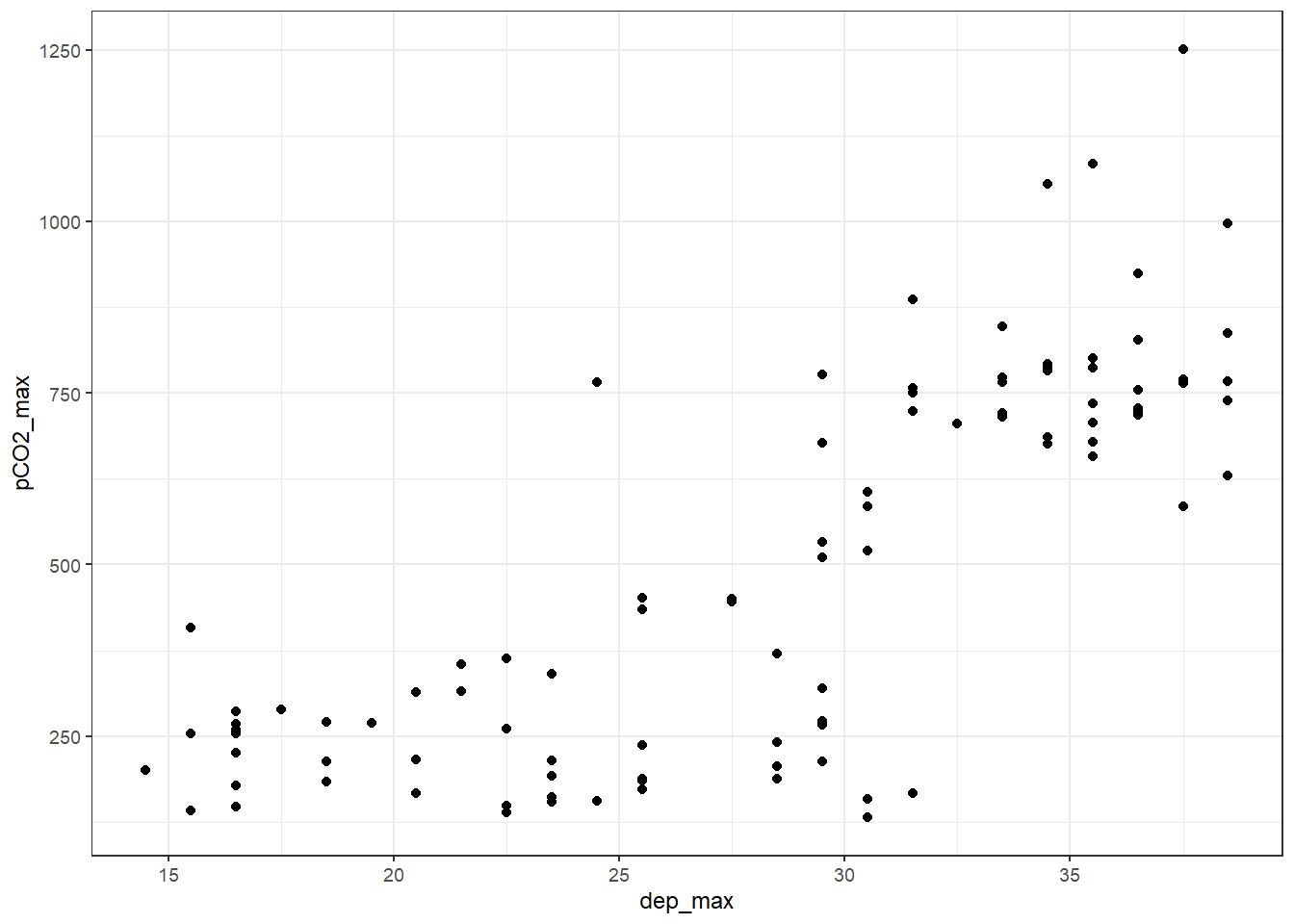

tm_grid <- full_join(tm_grid, tm_grid_stat)

meta <- read_csv(here::here("data/input/TinaV/Sensor",
                            "Sensor_meta.csv"),
                 col_types = cols(ID = col_character()))

tm_grid_stat <- full_join(meta, tm_grid_stat)

rm(tm_grid_stat, meta)

Summary metric are restricted to profiles that did not exceed:

• maximum sampling depth of 30 m
• pCO2 of 300 µatm
• Nr of missing depth grid levels of 2

# apply restrictions
tm_grid_shallow <- tm_grid %>% 
  filter(dep_max <= parameters$RT_stats_dep_max,
         pCO2_max <= parameters$RT_stats_pCO2_max,
         dep_grid <= parameters$RT_stats_dep) %>% 
  group_by(ID, station, tau_factor, correction) %>% 
  mutate(nr_na = sum(is.na(pCO2_delta))) %>% 
  ungroup() %>% 
  filter(nr_na < parameters$max_gap)

# calculate summary metrics up vs downcast
tm_grid_shallow_sum <- tm_grid_shallow %>% 
  mutate(pCO2_delta_abs = abs(pCO2_delta),
         pCO2_delta_rel_abs = abs(pCO2_delta_rel)) %>% 
  group_by(tau_factor, dep_grid, correction) %>% 
  summarise(mean         = mean(pCO2_delta, na.rm = TRUE),
            sd           = sd(pCO2_delta, na.rm = TRUE),
            mean_abs     = mean(pCO2_delta_abs, na.rm = TRUE),
            mean_rel     = mean(pCO2_delta_rel, na.rm = TRUE),
            sd_rel       = sd(pCO2_delta_rel, na.rm = TRUE),
            mean_rel_abs = mean(pCO2_delta_rel_abs, na.rm = TRUE)) %>% 
  ungroup() %>% 
  pivot_longer(cols = sd:mean_rel_abs,
               names_to = "estimate", values_to = "pCO2_delta")

# calculate summary metrics equilibrium comparison
tm_equi_delta_sum <- tm_equi_delta %>%
  mutate(pCO2_delta_equi_abs = abs(pCO2_delta_equi),
         pCO2_delta_equi_rel_abs = abs(pCO2_delta_equi_rel)) %>%
  group_by(correction, tau_factor) %>%
  summarise(mean         = mean(pCO2_delta_equi, na.rm = TRUE),
            mean_abs     = mean(pCO2_delta_equi_abs, na.rm = TRUE),
            mean_rel = mean(pCO2_delta_equi_rel, na.rm = TRUE),
            mean_rel_abs = mean(pCO2_delta_equi_rel_abs, na.rm = TRUE)) %>%
  ungroup() %>%
  pivot_longer(cols = mean:mean_rel_abs,
               names_to = "estimate", values_to = "dpCO2")

tm_grid_shallow_sum %>%
  filter(correction == "pCO2",
         estimate %in% c("mean_abs", "mean_rel_abs", "sd", "sd_rel")) %>%
  ggplot() +
  geom_vline(xintercept = 0) +
  geom_hline(yintercept = 20) +
  geom_vline(xintercept = c(10), col = "red") +
  geom_path(aes(pCO2_delta, dep_grid, col = as.factor(tau_factor))) +
  scale_y_reverse() +
  scale_color_discrete(name = "Tau factor") +
  labs(x = expression(Delta ~ italic(p)*CO[2] ~ (µatm)), y = "Depth intervals (1m)") +
  facet_grid(estimate ~ .)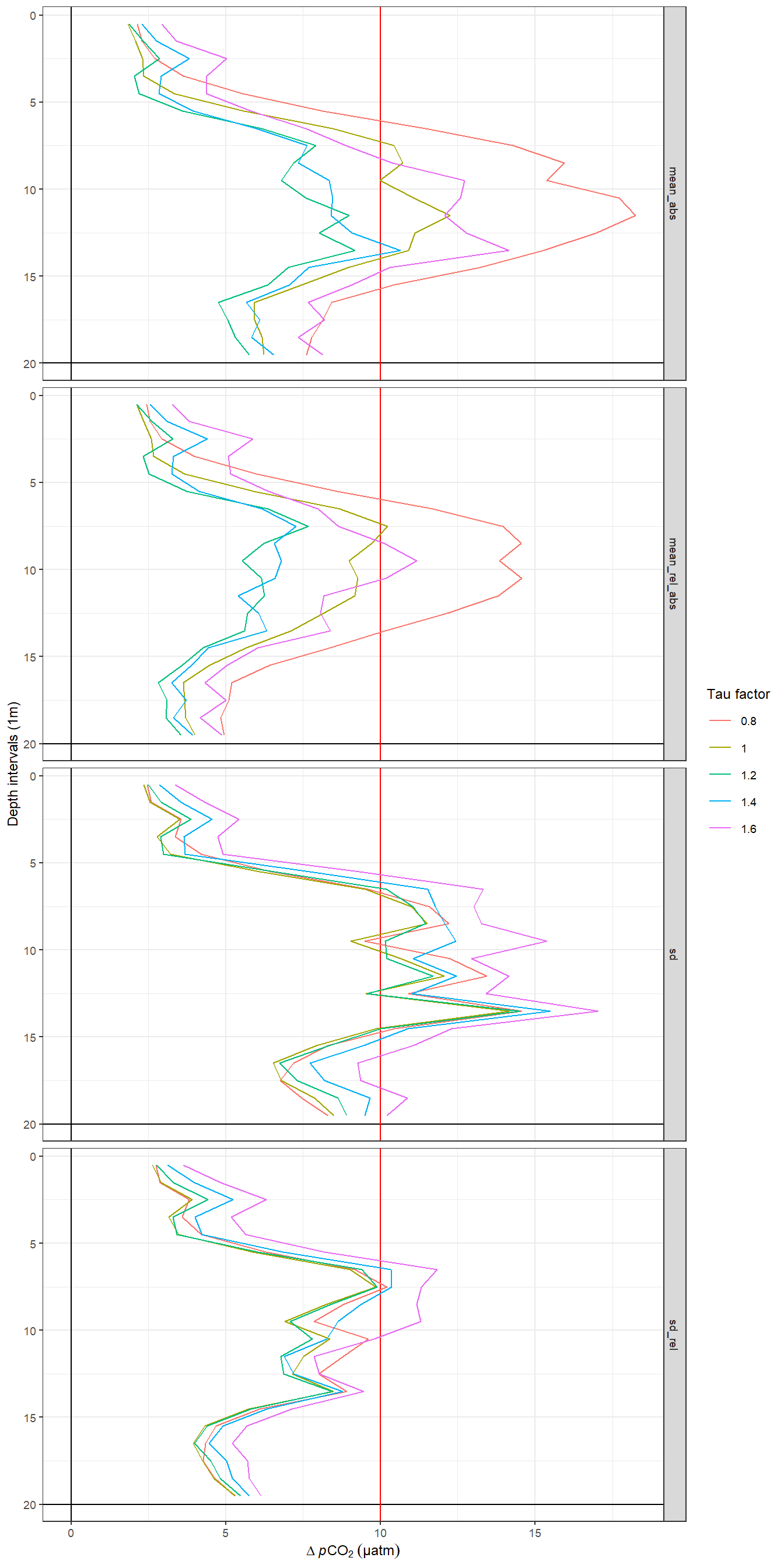

Offset between up- and downcast. Panel columns: Constant and T-dependent tau. Panel rows from top to bottom: Mean of absolute offset, mean of relative absolute offset, standard deviation of offset, standard deviation of relative offset.

Mean offset values calculated for the upper 5 and 20 m of the water column:

tm_grid_shallow_sum %>%
  filter(correction == "pCO2",
         estimate %in% c("mean_abs"),
         tau_factor == parameters$tau_factor_used,
         dep_grid < 5) %>% 
  summarise(dep_lim = 5,
            mean(pCO2_delta))

# A tibble: 1 x 2
  dep_lim `mean(pCO2_delta)`
    <dbl>              <dbl>
1       5               2.37

tm_grid_shallow_sum %>%
  filter(correction == "pCO2",
         estimate %in% c("mean_abs"),
         tau_factor == parameters$tau_factor_used,
         dep_grid < 20) %>% 
  summarise(dep_lim = 20,
            mean(pCO2_delta))

# A tibble: 1 x 2
  dep_lim `mean(pCO2_delta)`
    <dbl>              <dbl>
1      20               7.16

Likewise, we analyse the offset from the pCO₂ reference value:

tm_equi_delta_sum %>%
  filter(estimate %in% c("mean_abs", "mean_rel_abs")) %>%
  ggplot(aes(tau_factor, dpCO2, linetype = correction, shape = correction)) +
  geom_point() +
  geom_hline(yintercept = 0) +
  labs(x = "Tau factor", y = expression(Mean ~ Delta ~ italic(p)*CO[2])) +
  facet_wrap( ~ estimate)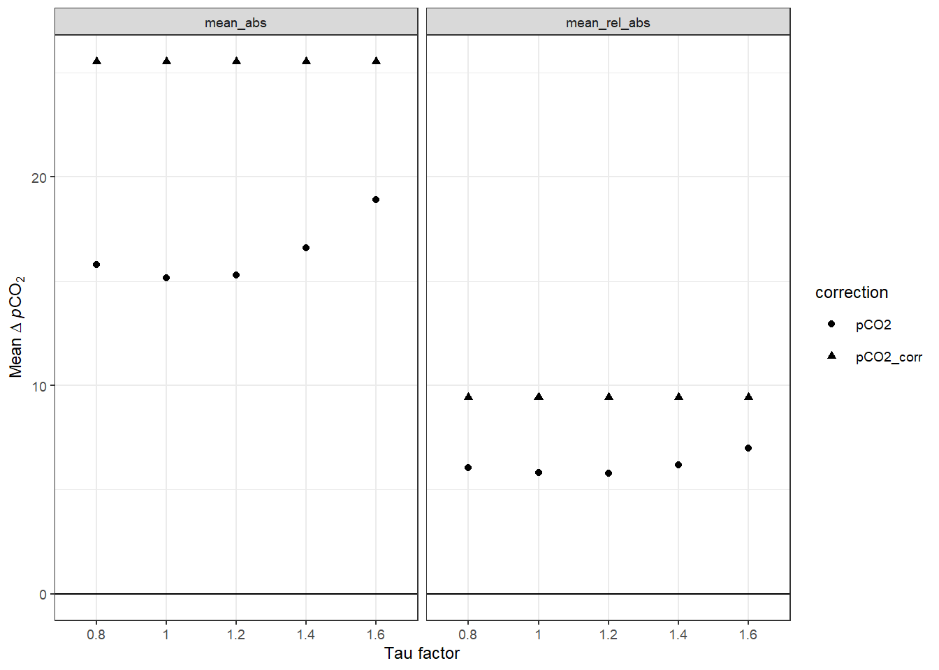

Mean pCO₂ offset from reference values as a function of the factor applied to tau. The lines between discrete tau factors result from the same analysis performed with high resolution of the tau factor. Left Panel: Mean absolute offset (µatm). Right panel: Mean relative offset (% of absolute value).

5.5 Summary plots

i_tau_factor <- "1"

cast_dep <- tm %>%
  filter(tau_factor == i_tau_factor) %>%
  pivot_longer(c(dep, pCO2_corr, pCO2),
               names_to = "parameter",
               values_to = "value")

cast_dep_equi <- tm_pCO2_equi %>%
  pivot_longer(c(dep, pCO2_corr), names_to = "parameter", values_to = "value")

tm_sub <- tm %>%
  filter(tau_factor == i_tau_factor)

tm_grid_sub <- tm_grid %>%
  filter(tau_factor == i_tau_factor)

max_duration <- round(max(cast_dep$duration) / 1000, 0) * 1000

pdf(
  file = here::here("output/Plots/response_time",
                    "all_plots.pdf"),
  onefile = TRUE,
  width = 7,
  height = 10
)

for (i_ID in unique(tm$ID)) {
  for (i_station in unique(tm$station)) {
    # i_ID <- unique(cast_dep$ID)[1]
    # i_station <- unique(cast_dep$station)[1]
    i_ID
    i_station
    
    if (nrow(cast_dep %>% filter(ID == i_ID, station == i_station)) > 0) {
      if (nrow(tm %>% filter(ID == i_ID, station == i_station)) > 0) {
        if (nrow(tm_grid %>% filter(ID == i_ID, station == i_station)) > 0) {
          cast_dep_equi_sub <- cast_dep_equi %>%
            filter(ID == i_ID,
                   station == i_station)
          
          p_time_series <- cast_dep %>%
            filter(ID == i_ID,
                   station == i_station) %>%
            ggplot(aes(duration, value, col = phase)) +
            geom_point(size = 0.5) +
            geom_point(data = cast_dep_equi_sub,
                       aes(duration, value),
                       col = "black") +
            scale_y_reverse() +
            scale_x_continuous(breaks = seq(0, 6000, 500)) +
            labs(title = str_c("ID: ", i_ID, " | Station: ", i_station)) +
            facet_grid(parameter ~ ., scales = "free_y") +
            theme_bw()
          
          p_profile <- tm_sub %>%
            filter(ID == i_ID,
                   station == i_station,
                   phase %in% c("up", "down")) %>%
            ggplot() +
            geom_path(aes(pCO2_corr, dep, linetype = phase, col = "raw")) +
            geom_path(aes(pCO2, dep, linetype = phase, col = "corrected")) +
            scale_y_reverse() +
            coord_cartesian(ylim = c(25, 0), xlim = c(70, 250)) +
            scale_color_brewer(palette = "Set1",
                               name = "",
                               guide = FALSE) +
            scale_linetype(guide = FALSE) +
            labs(y = "Depth [m]",
                 x = "pCO2",
                 title = "full res")
          
          
          tm_pCO2_equi_grid_sub <- tm_pCO2_equi_grid %>%
            filter(ID == i_ID,
                   station == i_station)
          
          p_profile_grid <- tm_grid_sub %>%
            filter(ID == i_ID,
                   station == i_station) %>%
            arrange(dep_grid) %>%
            ggplot() +
            geom_path(aes(down, dep_grid, col = correction, linetype = "down")) +
            geom_path(aes(up, dep_grid, col = correction, linetype = "up")) +
            geom_point(data = tm_pCO2_equi_grid_sub, aes(pCO2_equi, dep_grid)) +
            scale_y_reverse() +
            coord_cartesian(ylim = c(25, 0), xlim = c(70, 250)) +
            scale_linetype(name = "cast") +
            scale_color_brewer(palette = "Set1", direction = -1) +
            labs(x = "pCO2",
                 title = "1m grid") +
            theme(axis.title.y = element_blank(),
                  axis.text.y = element_blank())
          
          
          p_delta_abs <- tm_grid %>%
            filter(ID == i_ID,
                   station == i_station,
                   correction == "pCO2") %>%
            arrange(dep_grid) %>%
            ggplot(aes(pCO2_delta, dep_grid, col = as.factor(tau_factor))) +
            geom_path() +
            geom_point() +
            scale_y_reverse(breaks = seq(0, 40, 2)) +
            scale_color_discrete(name = "tau factor", guide = FALSE) +
            labs(x = "delta pCO2 [µatm]", y = "Depth [m]") +
            geom_vline(xintercept = 0) +
            geom_vline(xintercept = c(-10, 10), col = "red")
          
          p_delta_rel <- tm_grid %>%
            filter(ID == i_ID,
                   station == i_station,
                   correction == "pCO2") %>%
            arrange(dep_grid) %>%
            ggplot(aes(pCO2_delta_rel, dep_grid, col = as.factor(tau_factor))) +
            geom_path() +
            geom_point() +
            scale_y_reverse(breaks = seq(0, 40, 2)) +
            scale_color_discrete(name = "tau factor") +
            labs(x = "delta pCO2 [% of absolute value]", y = "Depth [m]") +
            geom_vline(xintercept = 0) +
            geom_vline(xintercept = c(-10, 10), col = "red") +
            theme(axis.title.y = element_blank(),
                  axis.text.y = element_blank())
          
          print(p_time_series / (p_profile |
                                   p_profile_grid) / (p_delta_abs | p_delta_rel))
          rm(p_time_series,
             p_profile,
             p_profile_grid,
             p_delta_abs,
             p_delta_rel)
          
        }
      }
    }
    
    
    
  }
}

dev.off()

rm(
  cast_dep,
  cast_dep_equi,
  cast_dep_equi_sub,
  i_station,
  i_ID,
  max_duration,
  tm_pCO2_equi_grid_sub
)

6 Conclusion

• Taking the temperature dependence of tau into account resulted in a slightly better agreement between up- and downcast, as well as downcast and reference value (Results not included above anymore)
• For most quality metrics we find improved agreement for slightly positive tau factor ranging from 1.04 - 1.24
• Still, the improvement by using a tau factor other then 1 is much lower than the standard deviation of the offset. Therefore, we assume that the improvement is not significant and choose to avoid the application of a tau factor for further analysis

7 Correct entire data set

Finally, the response time correction was applied to the full data set (not only profile data) based on the optimum parameterization determined above.

# # Response time correction approach after Bittig et al, 2018

# RT_corr <- function(c1, c0, dt, tau) {
#   (1 / (2 * ((1 + (
#     2 * tau / dt
#   )) ^ (-1)))) * (c1 - (1 - (2 * ((
#     1 + (2 * tau / dt)
#   ) ^ (
#     -1
#   )))) * c0)
# }

# Define function for response time correction after Fiedler et al, 2013

RT_corr <- function(c1, c0, dt, tau) {
(c1 - (c0 * exp(-dt/tau)) ) /
    (1 - exp(-dt/tau))
}


tm <-
  read_csv(
    here::here(
      "data/intermediate/_merged_data_files/merging_interpolation",
      "tm.csv"
    ),
    col_types = cols(
      ID = col_character(),
      pCO2_analog = col_double(),
      pCO2_corr = col_double(),
      Zero = col_factor(),
      Flush = col_factor(),
      Zero_counter = col_integer(),
      deployment = col_integer(),
      duration = col_double(),
      mixing = col_character(),
      lat = col_double(),
      lon = col_double()
    )
  )

tm <- tm %>%
  group_by(ID, station) %>%
  mutate(
    duration = as.numeric(date_time - min(date_time)),
    pump_power = if_else(date_time < ymd_hms("2018-07-17;13:08:34"), "1W", "8W")
  ) %>%
  arrange(date_time)


tau_fit <-
  read_csv(here::here(
    "data/intermediate/_merged_data_files/response_time",
    "tau_fit.csv"
  ))



# Assign T-dependent response time (tau) values
tau_fit <- tau_fit %>%
  rename(tau_intercept = `(Intercept)`, tau_slope = tem)

tm <- full_join(tm, tau_fit)

tm <- tm %>%
  mutate(tau = tau_intercept + tau_slope * tem) %>%
  select(-tau_intercept, -tau_slope)


# Prepare data set for RT correction

tm <- tm %>%
  group_by(ID, station) %>%
  arrange(date_time) %>%
  mutate(dt = as.numeric(as.character(date_time - lag(date_time)))) %>%
  ungroup()

# determine measurement frequency

freq <- tm %>%
  filter(dt < 13) %>%
  group_by(ID) %>%
  summarise(dt_mean = round(mean(dt, na.rm = TRUE), 0))

tm <- full_join(tm, freq)

# apply tau factor used
tm <- expand_grid(tm, tau_factor = parameters$tau_factor_used)

tm <- tm %>%
  mutate(tau_test = tau * tau_factor)


# Apply RT correction to entire data set

for (i_ID in unique(tm$ID)) {
  #i_ID <- "180716"
  
  freq_sub <- freq %>% filter(ID == i_ID) %>% pull(dt_mean)
  
  window <- 30 / freq_sub
  rolling_mean   <-
    rollify(~ mean(.x, na.rm = TRUE), window = window)
  
  tm_sub <- tm %>%
    filter(ID == i_ID) %>%
    group_by(station) %>%
    mutate(
      pCO2_RT = RT_corr(pCO2_corr, lag(pCO2_corr), dt, tau_test),
      pCO2_RT = if_else(pCO2_RT %in% c(Inf, -Inf), NaN, pCO2_RT),
      window = window,
      pCO2 = rolling_mean(pCO2_RT)
    ) %>%
    ungroup()
  
  # time shift RT corrected data
  shift <- as.integer(as.character(window / 2))
  
  tm_sub <- tm_sub %>%
    group_by(station) %>%
    mutate(pCO2 = lead(pCO2, shift)) %>%
    ungroup()
  
  
  if (exists("tm_corr")) {
    tm_corr <- bind_rows(tm_corr, tm_sub)
  }
  else{
    tm_corr <- tm_sub
  }
  
  rm(tm_sub, freq_sub, rolling_mean, shift, window)
  
}


rm(RT_corr, i_ID, freq)

tm_corr <- tm_corr %>%
  select(-c(tau, tau_factor, tau_test, window))

rm(tm)

7.1 Histogram

Below, histograms of RT corrected pCO₂ are shown, for selected ranges of pCO₂.

tm_corr %>% 
  ggplot(aes(pCO2)) +
  geom_histogram()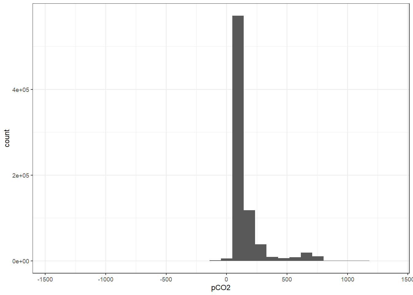

tm_corr %>% 
  filter(pCO2 < 0) %>% 
  ggplot(aes(pCO2)) +
  geom_histogram()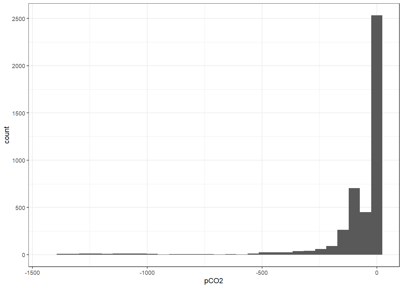

tm_corr %>% 
  filter(pCO2 < 200,
         pCO2 > 0) %>% 
  ggplot(aes(pCO2)) +
  geom_histogram()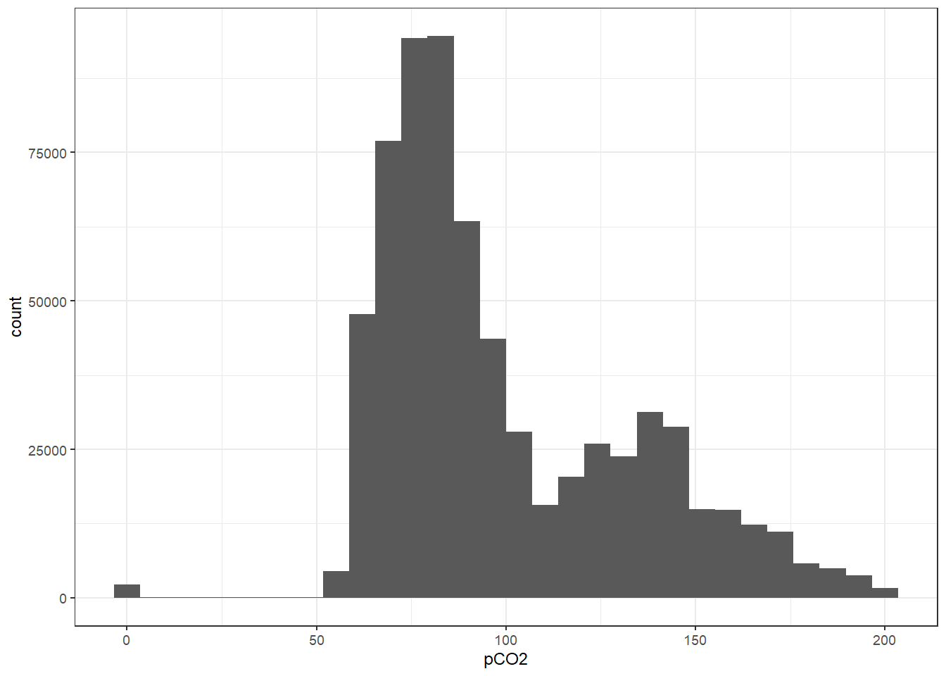

8 Write summary file

Response time corrected pCO₂ data with absolute values >50 are written to file for further analysis. Negative pCO₂ readings are considered artefacts of the response time correction.

tm_corr %>%
  filter(pCO2 > 50) %>% 
  write_csv(
    here::here(
      "data/intermediate/_merged_data_files/response_time",
      "tm_RT_all.csv"
    )
  )

9 Sensitivity considerations

A change in DIC of 1 µmol kg^-1 corresponds to a change in pCO₂ of around 1 µatm, in the Central Baltic Sea at a pCO₂ of around 100 µatm (summertime conditions).

df <- data.frame(cbind((c(1720)),
                       (c(7))))

Tem <- seq(5, 25, 5)
pCO2 <- seq(50, 500, 20)

df <- merge(df, Tem)
names(df) <- c("AT", "S", "Tem")

df <- merge(df, pCO2)
names(df) <- c("AT", "S", "Tem", "pCO2")

df$AT <- df$AT * 1e-6

df$DIC <-
  carb(
    flag = 24,
    var1 = df$pCO2,
    var2 = df$AT,
    S = df$S,
    T = df$Tem,
    k1k2 = "m10",
    kf = "dg",
    pHscale = "T"
  )[, 16]
df$pCO2.corr <-
  carb(
    flag = 15,
    var1 = df$AT,
    var2 = df$DIC,
    S = df$S,
    T = df$Tem,
    k1k2 = "m10",
    kf = "dg",
    pHscale = "T"
  )[, 9]

df$pCO2.2 <- df$pCO2.corr + 25
df$DIC.2 <-
  carb(
    flag = 24,
    var1 = df$pCO2.2,
    var2 = df$AT,
    S = df$S,
    T = df$Tem,
    k1k2 = "m10",
    kf = "dg",
    pHscale = "T"
  )[, 16]


df$ratio <- (df$pCO2.2 - df$pCO2.corr) / (df$DIC.2 * 1e6 - df$DIC * 1e6)

df %>%
  ggplot(aes(pCO2, ratio, col = as.factor(Tem))) +
  geom_line() +
  scale_color_viridis_d(option = "C", name = "Tem [°C]") +
  labs(x = expression(italic(p)*CO[2] ~ (µatm)),
       y = expression(Delta ~ italic(p)*CO[2] ~ "/" ~ Delta ~ DIC ~ (µatm ~ µmol ^ {
         -1
       } ~ kg))) +
  scale_y_continuous(limits = c(0, 8), breaks = seq(0, 10, 1))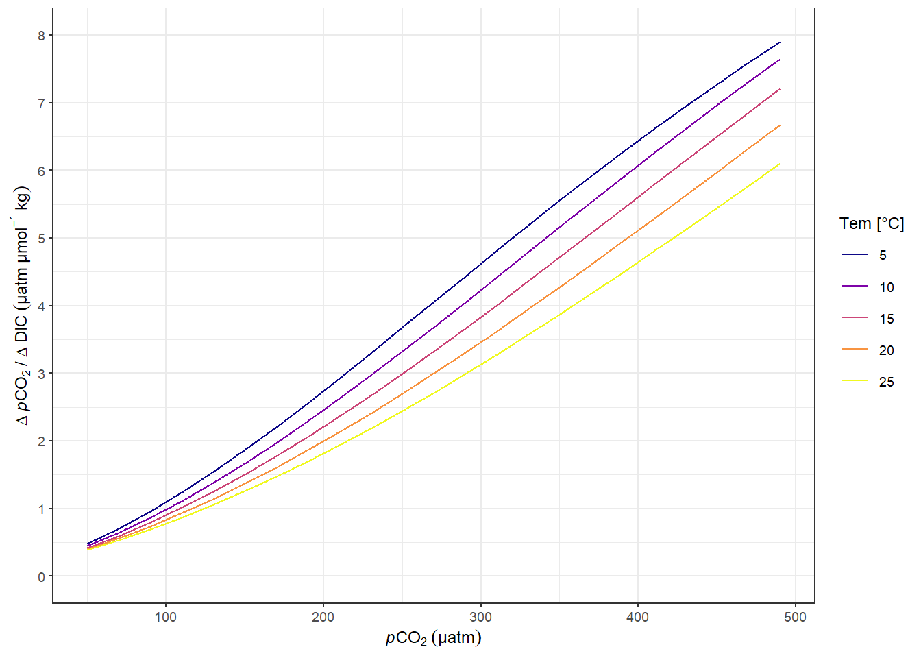

pCO₂ sensitivity to changes in DIC.

rm(df, Tem, pCO2)

Session information

sessionInfo()

R version 4.0.3 (2020-10-10)
Platform: x86_64-w64-mingw32/x64 (64-bit)
Running under: Windows 10 x64 (build 19042)

Matrix products: default

locale:
[1] LC_COLLATE=English_Germany.1252  LC_CTYPE=English_Germany.1252   
[3] LC_MONETARY=English_Germany.1252 LC_NUMERIC=C                    
[5] LC_TIME=English_Germany.1252    

attached base packages:
[1] stats     graphics  grDevices utils     datasets  methods   base     

other attached packages:
 [1] patchwork_1.1.1   tibbletime_0.1.6  lubridate_1.7.9.2 broom_0.7.5      
 [5] seacarb_3.2.14    oce_1.2-0         gsw_1.0-5         testthat_3.0.1   
 [9] forcats_0.5.0     stringr_1.4.0     dplyr_1.0.2       purrr_0.3.4      
[13] readr_1.4.0       tidyr_1.1.2       tibble_3.0.4      ggplot2_3.3.3    
[17] tidyverse_1.3.0   workflowr_1.6.2  

loaded via a namespace (and not attached):
 [1] httr_1.4.2         viridisLite_0.3.0  jsonlite_1.7.2     splines_4.0.3     
 [5] here_1.0.1         modelr_0.1.8       assertthat_0.2.1   highr_0.8         
 [9] cellranger_1.1.0   yaml_2.2.1         pillar_1.4.7       backports_1.2.1   
[13] lattice_0.20-41    glue_1.4.2         digest_0.6.27      RColorBrewer_1.1-2
[17] promises_1.1.1     rvest_0.3.6        colorspace_2.0-0   htmltools_0.5.0   
[21] httpuv_1.5.4       Matrix_1.2-18      pkgconfig_2.0.3    haven_2.3.1       
[25] scales_1.1.1       whisker_0.4        later_1.1.0.1      git2r_0.27.1      
[29] mgcv_1.8-33        generics_0.1.0     farver_2.0.3       ellipsis_0.3.1    
[33] withr_2.3.0        cli_2.2.0          magrittr_2.0.1     crayon_1.3.4      
[37] readxl_1.3.1       evaluate_0.14      ps_1.5.0           fs_1.5.0          
[41] fansi_0.4.1        nlme_3.1-149       xml2_1.3.2         tools_4.0.3       
[45] hms_0.5.3          lifecycle_0.2.0    munsell_0.5.0      reprex_0.3.0      
[49] compiler_4.0.3     rlang_0.4.10       grid_4.0.3         rstudioapi_0.13   
[53] labeling_0.4.2     rmarkdown_2.6      gtable_0.3.0       DBI_1.1.0         
[57] R6_2.5.0           knitr_1.30         utf8_1.1.4         rprojroot_2.0.2   
[61] stringi_1.5.3      Rcpp_1.0.5         vctrs_0.3.6        dbplyr_2.0.0      
[65] tidyselect_1.1.0   xfun_0.19