Last updated: 2021-05-18

Checks: 7 0

Knit directory: BloomSail/

This reproducible R Markdown analysis was created with workflowr (version 1.6.2). The Checks tab describes the reproducibility checks that were applied when the results were created. The Past versions tab lists the development history.

R Markdown file: up-to-date

Great! Since the R Markdown file has been committed to the Git repository, you know the exact version of the code that produced these results.

Environment: empty

Great job! The global environment was empty. Objects defined in the global environment can affect the analysis in your R Markdown file in unknown ways. For reproduciblity it’s best to always run the code in an empty environment.

Seed: set.seed(20191021)

The command set.seed(20191021) was run prior to running the code in the R Markdown file. Setting a seed ensures that any results that rely on randomness, e.g. subsampling or permutations, are reproducible.

Session information: recorded

Great job! Recording the operating system, R version, and package versions is critical for reproducibility.

Cache: none

Nice! There were no cached chunks for this analysis, so you can be confident that you successfully produced the results during this run.

File paths: relative

Great job! Using relative paths to the files within your workflowr project makes it easier to run your code on other machines.

Repository version: 00a2574

Great! You are using Git for version control. Tracking code development and connecting the code version to the results is critical for reproducibility.

The results in this page were generated with repository version 00a2574. See the Past versions tab to see a history of the changes made to the R Markdown and HTML files.

Note that you need to be careful to ensure that all relevant files for the analysis have been committed to Git prior to generating the results (you can use wflow_publish or wflow_git_commit). workflowr only checks the R Markdown file, but you know if there are other scripts or data files that it depends on. Below is the status of the Git repository when the results were generated:


Ignored files:
    Ignored:    .Rhistory
    Ignored:    .Rproj.user/
    Ignored:    data/
    Ignored:    output/Plots/Figures_publication/.tmp.drivedownload/

Untracked files:
    Untracked:  data_os-2020-120_submission.zip

Unstaged changes:
    Modified:   code/Workflowr_project_managment.R
    Modified:   output/Plots/Figures_publication/Appendix/Fig_A1.pdf
    Modified:   output/Plots/Figures_publication/Appendix/Fig_A2.pdf
    Modified:   output/Plots/Figures_publication/Appendix/Fig_B1.pdf
    Modified:   output/Plots/Figures_publication/Appendix/Fig_B2.pdf
    Modified:   output/Plots/Figures_publication/Appendix/Fig_B2.png
    Modified:   output/Plots/Figures_publication/Appendix/Fig_C1.pdf
    Modified:   output/Plots/Figures_publication/Appendix/Fig_C2.pdf
    Modified:   output/Plots/Figures_publication/Appendix/Fig_C3.pdf
    Modified:   output/Plots/Figures_publication/Appendix/Fig_C4.pdf
    Modified:   output/Plots/Figures_publication/Article/Fig_1.pdf
    Modified:   output/Plots/Figures_publication/Article/Fig_2.pdf
    Modified:   output/Plots/Figures_publication/Article/Fig_3.pdf
    Modified:   output/Plots/Figures_publication/Article/Fig_4.pdf
    Modified:   output/Plots/Figures_publication/Article/Fig_5.pdf
    Modified:   output/Plots/Figures_publication/Article/Fig_6.pdf
    Modified:   output/Plots/NCP_best_guess/tm_profiles_ID_pCO2_tem_sal_CT.pdf
    Modified:   output/Plots/NCP_best_guess/tm_profiles_pCO2_tem_sal_CT.pdf
    Modified:   output/Plots/response_time/all_plots.pdf
    Modified:   output/Plots/response_time/profiles_pCO2.pdf
    Modified:   output/Plots/response_time/profiles_pCO2_delta_grid.pdf
    Modified:   output/Plots/response_time/profiles_pCO2_delta_rel_grid.pdf
    Modified:   output/Plots/response_time/profiles_pCO2_grid.pdf
    Modified:   output/Plots/response_time/tau_determination_pCO2_corr_flushperiods_nls.pdf
    Modified:   output/Plots/response_time/time_series_depth_pCO2_corr_by_profile.pdf

Note that any generated files, e.g. HTML, png, CSS, etc., are not included in this status report because it is ok for generated content to have uncommitted changes.

These are the previous versions of the repository in which changes were made to the R Markdown (analysis/NCP_reconstruction.Rmd) and HTML (docs/NCP_reconstruction.html) files. If you’ve configured a remote Git repository (see ?wflow_git_remote), click on the hyperlinks in the table below to view the files as they were in that past version.

File	Version	Author	Date	Message
html	00a2574	jens-daniel-mueller	2021-05-10	Build site.
html	0e06676	jens-daniel-mueller	2021-05-10	Build site.
Rmd	f5ceb42	jens-daniel-mueller	2021-05-10	removed grid lines
html	61e452c	jens-daniel-mueller	2021-04-16	Build site.
html	8734af2	jens-daniel-mueller	2021-03-30	Build site.
Rmd	3349e44	jens-daniel-mueller	2021-03-30	revised figure according to RC1
html	f63cc06	jens-daniel-mueller	2021-03-30	Build site.
Rmd	d5f897e	jens-daniel-mueller	2021-03-30	revised figure according to RC1
html	2f64f92	jens-daniel-mueller	2021-03-30	Build site.
Rmd	23acb8c	jens-daniel-mueller	2021-03-30	revised figure according to RC1
html	16c93d2	jens-daniel-mueller	2021-03-30	Build site.
Rmd	7ba53a1	jens-daniel-mueller	2021-03-30	revised figure according to RC1
html	5f4fb9a	jens-daniel-mueller	2021-02-20	Build site.
Rmd	031f46a	jens-daniel-mueller	2021-02-20	rerun with early exclusion of negative pCO2
html	516b294	jens-daniel-mueller	2021-02-18	Build site.
Rmd	233bbc1	jens-daniel-mueller	2021-02-18	rerun all with empty folders
html	184f00b	jens-daniel-mueller	2021-02-18	Build site.
Rmd	955ac1d	jens-daniel-mueller	2021-02-18	cleaning
html	43f9d47	jens-daniel-mueller	2021-02-18	Build site.
Rmd	54ddb86	jens-daniel-mueller	2021-02-18	cleaning
html	3d08cda	jens-daniel-mueller	2021-02-18	Build site.
Rmd	c909ee0	jens-daniel-mueller	2021-02-18	cleaning
html	67dd4d7	jens-daniel-mueller	2021-02-18	Build site.
Rmd	cc7316f	jens-daniel-mueller	2021-02-18	cleaning
html	7014ec6	jens-daniel-mueller	2021-02-18	Build site.
Rmd	c832869	jens-daniel-mueller	2021-02-18	cleaning
html	3e94656	jens-daniel-mueller	2021-02-18	Build site.
Rmd	93a094c	jens-daniel-mueller	2021-02-18	cleaning
html	189f202	jens-daniel-mueller	2021-02-16	Build site.
Rmd	06d5293	jens-daniel-mueller	2021-02-16	cleaning
html	0af0021	jens-daniel-mueller	2021-02-15	Build site.
Rmd	4878a06	jens-daniel-mueller	2021-02-15	cleaning
html	70a8950	jens-daniel-mueller	2021-02-11	Build site.
Rmd	4bdeb1f	jens-daniel-mueller	2021-02-11	rerun all with empty folders
html	8051798	jens-daniel-mueller	2021-02-10	Build site.
Rmd	9477a18	jens-daniel-mueller	2021-02-10	rerun all with empty folders
html	b70ce3a	jens-daniel-mueller	2021-02-04	Build site.
Rmd	f8ff3d7	jens-daniel-mueller	2021-02-04	resized figures
html	2394871	jens-daniel-mueller	2021-02-03	Build site.
Rmd	6747fd9	jens-daniel-mueller	2021-02-03	resized figures
html	d6c7395	jens-daniel-mueller	2021-02-02	Build site.
Rmd	4de153f	jens-daniel-mueller	2021-02-02	renamed figures
html	289b763	jens-daniel-mueller	2021-01-30	Build site.
Rmd	b470c95	jens-daniel-mueller	2021-01-30	resized figures
html	6adb9ab	jens-daniel-mueller	2021-01-29	Build site.
Rmd	54ec4b0	jens-daniel-mueller	2021-01-29	renamed appendix figures
html	2677b39	jens-daniel-mueller	2021-01-28	Build site.
Rmd	3eae87b	jens-daniel-mueller	2021-01-28	modified figs
html	c5fc34c	jens-daniel-mueller	2021-01-22	Build site.
Rmd	f656a73	jens-daniel-mueller	2021-01-22	all figs revised
html	a7950fd	jens-daniel-mueller	2021-01-22	Build site.
Rmd	88fcb00	jens-daniel-mueller	2021-01-22	modified figs
html	cde4f1d	jens-daniel-mueller	2021-01-08	Build site.
Rmd	7cd025c	jens-daniel-mueller	2021-01-08	modified figs
html	e55d103	jens-daniel-mueller	2021-01-05	Build site.
Rmd	f31d3e2	jens-daniel-mueller	2021-01-05	revised figure 4 and 6
html	0bc930a	jens-daniel-mueller	2021-01-05	Build site.
Rmd	1fb97c7	jens-daniel-mueller	2021-01-05	revised figure 6
html	4277235	jens-daniel-mueller	2021-01-05	Build site.
Rmd	58c1637	jens-daniel-mueller	2021-01-05	new Fig_AX names, A5 added
html	2a105b2	jens-daniel-mueller	2020-11-04	Build site.
Rmd	2c4509a	jens-daniel-mueller	2020-11-04	added panel annotation
html	7e29c30	jens-daniel-mueller	2020-11-02	Build site.
Rmd	7e5a700	jens-daniel-mueller	2020-11-02	renamed and revised figures for publication
html	61753ef	jens-daniel-mueller	2020-10-30	Build site.
Rmd	0628954	jens-daniel-mueller	2020-10-30	renamed plot output
html	838a9c3	jens-daniel-mueller	2020-10-30	Build site.
Rmd	37582a4	jens-daniel-mueller	2020-10-30	updated plot
html	bef182d	jens-daniel-mueller	2020-10-30	Build site.
Rmd	0b9ca47	jens-daniel-mueller	2020-10-30	updated plot
html	9a3f42a	jens-daniel-mueller	2020-10-24	Build site.
html	dd86a70	jens-daniel-mueller	2020-10-21	Build site.
Rmd	0711e3e	jens-daniel-mueller	2020-10-21	display MLD mean and sd values
html	05248bf	jens-daniel-mueller	2020-10-20	Build site.
html	1c4fe8e	jens-daniel-mueller	2020-10-20	table with time series in depth intervals added
html	6896725	jens-daniel-mueller	2020-10-01	Build site.
html	9f66019	jens-daniel-mueller	2020-10-01	Build site.
html	27c5431	jens-daniel-mueller	2020-09-29	Build site.
Rmd	2e0f902	jens-daniel-mueller	2020-09-29	all parameters separate, rebuild
html	1d01685	jens-daniel-mueller	2020-09-28	Build site.
html	1278900	jens-daniel-mueller	2020-09-25	Build site.
html	904f0f7	jens-daniel-mueller	2020-09-23	Build site.
html	66bf52a	jens-daniel-mueller	2020-09-23	Build site.
Rmd	0c8eed6	jens-daniel-mueller	2020-09-23	included postprocessed cleaned data
html	e4797a2	jens-daniel-mueller	2020-07-01	Build site.
Rmd	857208b	jens-daniel-mueller	2020-07-01	update NCP recon figure
html	c919fb7	jens-daniel-mueller	2020-06-29	Build site.
Rmd	1461cb6	jens-daniel-mueller	2020-06-29	Fig update for talk
html	603af23	jens-daniel-mueller	2020-05-25	Build site.
html	3414c23	jens-daniel-mueller	2020-05-25	Build site.
html	9eb7215	jens-daniel-mueller	2020-05-25	Build site.
Rmd	80a7e08	jens-daniel-mueller	2020-05-25	Removed separate BloomSail and fm+gt reconstruction
html	c5cf8de	jens-daniel-mueller	2020-05-25	Build site.
Rmd	2b97ae3	jens-daniel-mueller	2020-05-25	added gas flux to reconstructed iCT
html	4dd0f4f	jens-daniel-mueller	2020-05-25	Build site.
Rmd	f7f0983	jens-daniel-mueller	2020-05-25	added gas flux to reconstructed iCT
html	1b366c4	jens-daniel-mueller	2020-05-25	Build site.
Rmd	eef261f	jens-daniel-mueller	2020-05-25	TPD CPD appendix plots
html	9166c1d	jens-daniel-mueller	2020-05-20	Build site.
Rmd	ef99640	jens-daniel-mueller	2020-05-20	finalized reconstruction approach
html	1e15837	jens-daniel-mueller	2020-05-20	Build site.
Rmd	2378108	jens-daniel-mueller	2020-05-20	finalized iCT reconstruction
html	6aad8d7	jens-daniel-mueller	2020-05-19	Build site.
Rmd	d7aa227	jens-daniel-mueller	2020-05-19	finalized integration depth estimates
html	ae5779d	jens-daniel-mueller	2020-05-19	Build site.
Rmd	5651fe5	jens-daniel-mueller	2020-05-19	removed deep warming signal for z_pen determination
html	6e3d899	jens-daniel-mueller	2020-05-19	Build site.
Rmd	0ba33ec	jens-daniel-mueller	2020-05-19	cleaned NCP reconstruction IV
html	7f4066e	jens-daniel-mueller	2020-05-19	Build site.
Rmd	536cb1a	jens-daniel-mueller	2020-05-19	cleaned NCP reconstruction III
html	dd7e745	jens-daniel-mueller	2020-05-19	Build site.
Rmd	33c4313	jens-daniel-mueller	2020-05-19	cleaned NCP reconstruction II
html	57b5f60	jens-daniel-mueller	2020-05-19	Build site.
Rmd	fa8ce00	jens-daniel-mueller	2020-05-19	cleaned NCP reconstruction
html	6fcea7b	jens-daniel-mueller	2020-05-18	Build site.
Rmd	09ccf10	jens-daniel-mueller	2020-05-18	merged tm and gt NCP reconstruction

library(tidyverse)
library(ncdf4)
library(seacarb)
library(oce)
library(patchwork)
library(lubridate)
library(metR)

1 Scope of this script

In order to test how well the depth-integrated C_T* estimates can be reproduced if only surface CO₂ data were available, the following reconstruction approaches were tested:

Mixed layer depth: Integration of surface observation across the MLD, assuming homogeneous vertical patterns
C_T profile reconstruction: Vertical reconstruction of incremental C_T changes based on profiles of incremental changes in temperature
Temperature penetration depth: Integration of surface observation across the temperature penetration depth, assuming similar vertical extension as for C_T drawdown.

Note: The reconstruction of C_T* profiles and the integration across the temperature penetration depth should produce very similar results. However, the latter avoids to create misinterpretable information about the vertical distribution of C_T*.

The integration depth parameterizations were tested on two data sets, namely:

BloomSail observations, restricted to C_T* data in surface water
SOOP Finnmaid pCO₂ + vertical hydrographical data from GETM model

date_CT_min <- ymd_hms("2018-07-24 07:58:29")
date_tem_max <- ymd_hms("2018-08-04 00:00:00")

2 BloomSail

1m gridded, downcast profiles were used.

Mean CO₂ data from upper 6 meters were used as surface values.

# read data
tm_profiles_ID <-
  read_csv(
    here::here(
      "data/intermediate/_merged_data_files/NCP_best_guess",
      "tm_profiles_ID.csv"
    )
  )

tm_profiles_ID <- tm_profiles_ID %>% 
  select(-c(date_ID))

# calculate cumulative changes

tm_profiles_ID_long <- tm_profiles_ID %>%
  select(-c(pCO2, sal)) %>% 
  pivot_longer(c("tem", "CT_star"), values_to = "value", names_to = "var") %>% 
  group_by(var, dep) %>%
  arrange(date_time_ID) %>%
  mutate(date_time_ID_diff = as.numeric(date_time_ID - lag(date_time_ID)),
         value_diff = value     - lag(value, default = first(value)),
         value_diff_daily = value_diff / date_time_ID_diff,
         value_cum = cumsum(value_diff)) %>% 
  ungroup()

2.1 TPD and CPD

Temperature penetration depth (TPD) and C_T* penetration depth (CPD) were investigated based on the BloomSail data.

2.1.1 Cumulative profile July 9

# subset date for cumulative assesment
tm_profiles_ID_long_day <- tm_profiles_ID_long %>%
  filter(ID == 180709)

# calculate integrated value of pos/neg changes for Temp/CT*
# and relative contribution with increasing water depth 
tm_profiles_ID_long_day_dep <- tm_profiles_ID_long_day %>%
  select(var, dep, value_cum) %>%
  mutate(
    value_cum = if_else(value_cum > 0 & var == "CT_star",
                        NaN, value_cum),
    value_cum = if_else(value_cum < 0 & var == "tem",
                        NaN, value_cum)
  ) %>%
  group_by(var) %>%
  arrange(dep) %>%
  mutate(
    value_cum_i = sum(value_cum, na.rm = TRUE),
    value_cum_dep = cumsum(value_cum),
    value_cum_i_rel = value_cum_dep / value_cum_i * 100
  ) %>%
  ungroup()

# cumulative integrated values
value_cum <- tm_profiles_ID_long_day_dep %>%
  group_by(var) %>%
  summarise(value_cum_i = mean(value_cum_i)) %>%
  ungroup()

# cumulative surface values
value_surface <- tm_profiles_ID_long_day %>%
  select(var, dep, value_cum) %>%
  filter(dep < parameters$surface_dep) %>%
  group_by(var) %>%
  summarise(value_surface = mean(value_cum)) %>%
  ungroup()

# calculate penentration depth for T and C
PD <- full_join(value_cum, value_surface)
PD <- PD %>%
  mutate(PD = value_cum_i / value_surface)

rm(value_cum, value_surface)

p_tm_profiles_ID_long <- tm_profiles_ID_long_day %>%
  arrange(dep) %>%
  ggplot(aes(value_cum, dep)) +
  geom_hline(aes(yintercept = parameters$i_dep_lim, col = "integration")) +
  geom_hline(data = PD, aes(yintercept = PD, col = "penetration")) +
  geom_vline(xintercept = 0) +
  geom_point() +
  geom_path() +
  scale_y_reverse() +
  scale_color_brewer(palette = "Dark2", guide = FALSE) +
  labs(y = "Depth (m)", x = "Cumulative change") +
  theme(legend.position = "left") +
  facet_wrap(var ~ ., ncol = 1, scales = "free_x")

p_tm_profiles_ID_long_rel <- tm_profiles_ID_long_day_dep %>%
  ggplot(aes(value_cum_i_rel, dep)) +
  geom_hline(aes(yintercept = parameters$i_dep_lim, col = "integration")) +
  geom_hline(data = PD, aes(yintercept = PD, col = "penetration")) +
  geom_vline(xintercept = 90) +
  geom_point() +
  geom_line() +
  scale_y_reverse(limits = c(25, 0)) +
  scale_color_brewer(palette = "Dark2", name = "Depth") +
  scale_x_continuous(limits = c(0, NA)) +
  labs(x = "Relative contribution (%)") +
  facet_wrap(var ~ ., ncol = 1, scales = "free_x") +
  theme(axis.title.y = element_blank())

p_tm_profiles_ID_long + p_tm_profiles_ID_long_rel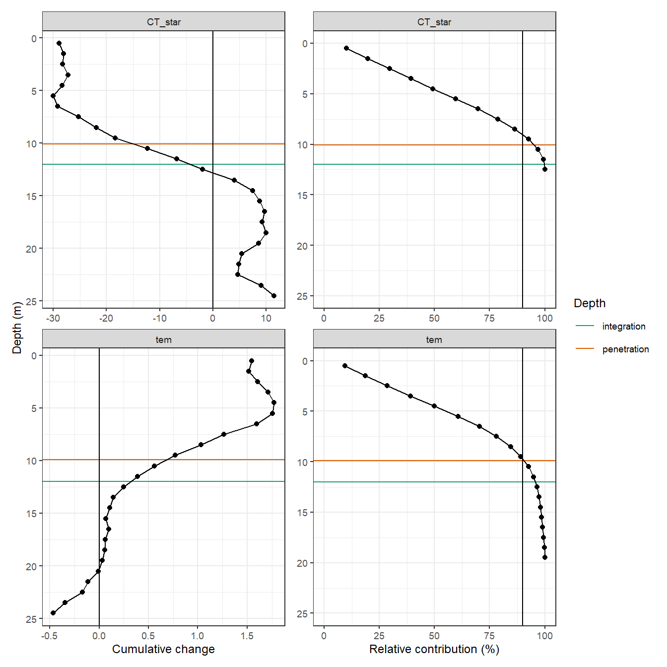

PD

# A tibble: 2 x 4
  var     value_cum_i value_surface    PD
  <chr>         <dbl>         <dbl> <dbl>
1 CT_star      -286.         -28.5  10.1 
2 tem            16.3          1.65  9.90

rm(tm_profiles_ID_long_day_dep,
   p_tm_profiles_ID_long,
   p_tm_profiles_ID_long_rel)

2.1.2 Incremental profile July 9

col_value <- "red"

p_CT_star <-
  tm_profiles_ID_long_day %>%
  filter(var == "CT_star") %>%
  arrange(dep) %>%
  ggplot() +
  geom_col(
    data = tm_profiles_ID_long_day %>%
      filter(var == "CT_star", value_diff_daily < 0),
    aes(x = value_diff_daily, y = dep),
    width = 1,
    alpha = 0.2,
    orientation = "y"
  ) +
  geom_vline(xintercept = 0) +
  scale_y_reverse(expand = c(0, 0)) +
  annotate(
    "text",
    x = -6,
    y = 11,
    label = "CPD",
    col = col_value,
    size = geom_text_size
  ) +
  annotate(
    "text",
    x = -3.5,
    y = 2.5,
    label = "Integrated\nchange",
    size = geom_text_size
  ) +
  geom_point(aes(value_diff_daily, dep)) +
  geom_path(aes(value_diff_daily, dep)) +
  geom_hline(data = PD %>% filter(var == "CT_star"),
             aes(yintercept = PD),
             col = col_value) +
  labs(y = "Depth (m)", x = expression(paste(Delta ~ C[T], "*") ~ (µmol ~ kg ^ {
    -1
  }))) +
  theme(
    legend.title = element_blank(),
    axis.text.y = element_blank(),
    axis.ticks.y = element_blank(),
    axis.title.y = element_blank(),
    panel.grid.minor = element_blank()
  )

p_tem <-
  tm_profiles_ID_long_day %>%
  filter(var == "tem") %>%
  arrange(dep) %>%
  ggplot() +
  geom_col(
    data = tm_profiles_ID_long_day %>%
      filter(var == "tem", value_diff_daily > 0),
    aes(x = value_diff_daily, y = dep),
    width = 1,
    alpha = 0.2,
    orientation = "y"
  ) +
  geom_vline(xintercept = 0) +
  scale_y_reverse(expand = c(0, 0)) +
  annotate(
    "text",
    x = 0.4,
    y = 11,
    label = "TPD",
    col = col_value,
    size = geom_text_size
  ) +
  annotate(
    "text",
    x = 0.2,
    y = 2.5,
    label = "Integrated\nchange",
    size = geom_text_size
  ) +
  geom_point(aes(value_diff_daily, dep)) +
  geom_path(aes(value_diff_daily, dep)) +
  geom_hline(data = PD %>% filter(var == "tem"),
             aes(yintercept = PD),
             col = col_value) +
  labs(y = "Depth (m)", x = expression(Delta ~ Temp. ~ (degree * C))) +
  theme(legend.title = element_blank(),
        panel.grid.minor = element_blank())

p_tem + p_CT_star +
  plot_layout(guides = 'collect') +
  plot_annotation(tag_levels = 'a')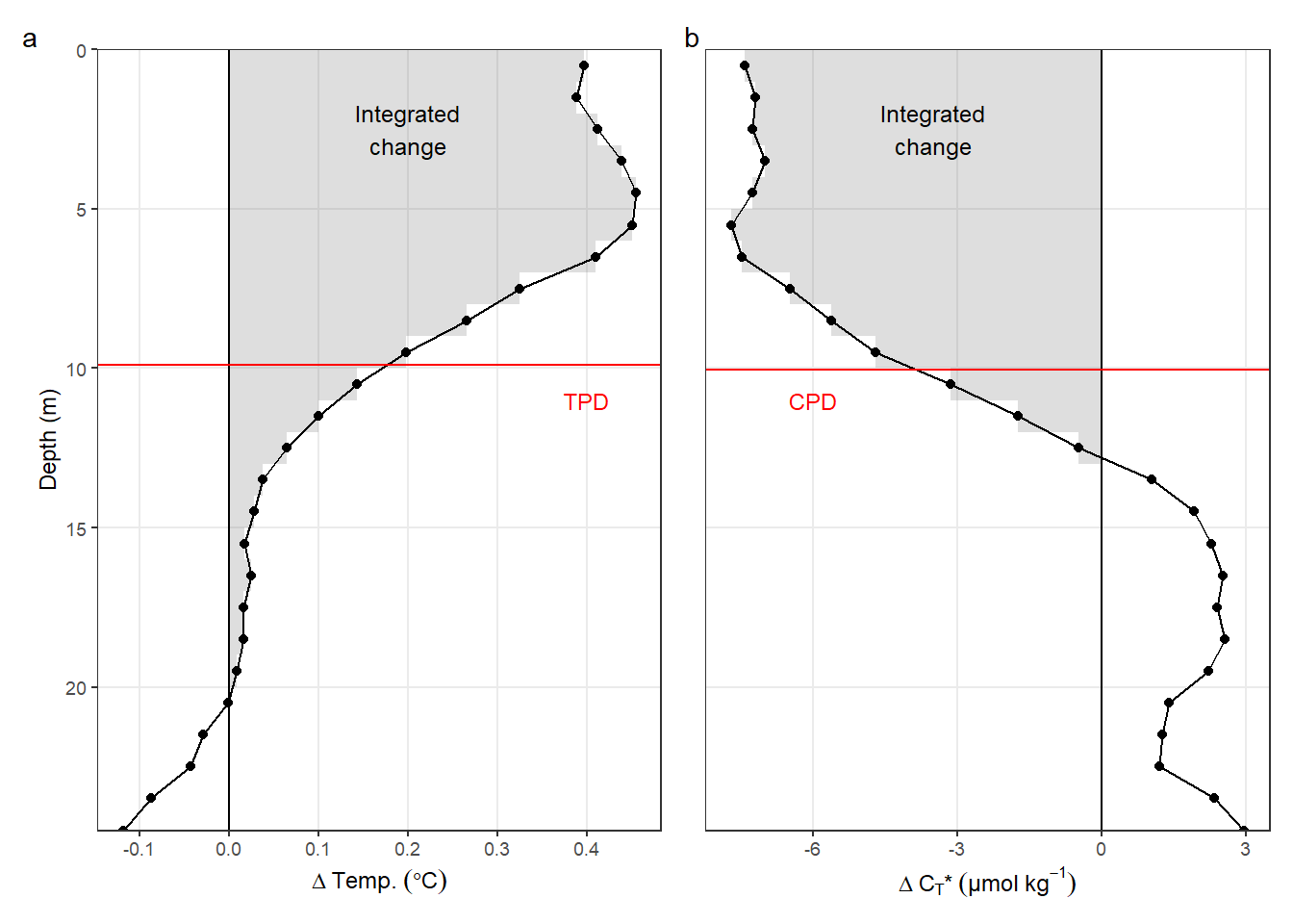

ggsave(
  here::here("output/Plots/Figures_publication/appendix",
             "Fig_C4.pdf"),
  width = 120,
  height = 110,
  dpi = 300,
  units = "mm"
)

ggsave(
  here::here("output/Plots/Figures_publication/appendix",
             "Fig_C4.png"),
  width = 120,
  height = 110,
  dpi = 300,
  units = "mm"
)

rm(PD, tm_profiles_ID_long_day, p_tem, p_CT_star, col_value)

2.1.3 Incremental time series

A time series of TPD and CPD was calculated, based on the incremental (ie from cruise day to cruise day) changes of temperature / C_T*, taking only pos. / neg. changes of both parameters into account.

# surface values
diff_surface <- tm_profiles_ID_long %>%
  filter(dep < parameters$surface_dep) %>%
  group_by(ID, var) %>%
  summarise(value_diff_surface = mean(value_diff, na.rm = TRUE)) %>%
  ungroup() %>%
  mutate(
    value_diff_surface = if_else(value_diff_surface > 0 & var == "CT_star",
                                 NaN, value_diff_surface),
    value_diff_surface = if_else(value_diff_surface < 0 &
                                   var == "tem",
                                 NaN, value_diff_surface)
  )

tm_profiles_ID_long <- full_join(tm_profiles_ID_long, diff_surface)
rm(diff_surface)

# calculate penetration depths for T and C
PD <- tm_profiles_ID_long %>%
  mutate(
    value_diff = if_else(value_diff > 0 & var == "CT_star",
                         NaN, value_diff),
    value_diff = if_else(value_diff < 0 & var == "tem",
                         NaN, value_diff)
  ) %>%
  group_by(var, ID, date_time_ID) %>%
  summarise(
    value_diff_int = sum(value_diff, na.rm = TRUE),
    value_diff_surface = mean(value_diff_surface, na.rm = TRUE)
  ) %>%
  ungroup() %>%
  mutate(i_dep = value_diff_int / value_diff_surface)

# calculate temporal mean
PD_mean <- PD %>%
  group_by(var) %>%
  summarise(i_dep_mean = mean(i_dep, na.rm = TRUE),
            i_dep_sd = sd(i_dep, na.rm = TRUE)) %>%
  ungroup()

p_surface <- PD %>%
  ggplot(aes(date_time_ID, value_diff_surface)) +
  geom_hline(yintercept = 0) +
  geom_line() +
  geom_point() +
  scale_y_reverse(name = "Change surface value") +
  scale_x_datetime(breaks = "week", date_labels = "%d %b") +
  scale_color_brewer(palette = "Set1", direction = -1) +
  theme(axis.title.x = element_blank(),
        legend.title = element_blank()) +
  facet_grid(var ~ ., scales = "free_y")

p_integrated <- PD %>%
  ggplot(aes(date_time_ID, value_diff_int)) +
  geom_hline(yintercept = 0) +
  geom_line() +
  geom_point() +
  scale_y_reverse(name = "Change integrated value") +
  scale_x_datetime(breaks = "week", date_labels = "%d %b") +
  scale_color_brewer(palette = "Set1", direction = -1) +
  theme(axis.title.x = element_blank(),
        legend.title = element_blank()) +
  facet_grid(var ~ ., scales = "free_y")

p_pen_dep <- PD %>%
  ggplot(aes(date_time_ID, i_dep, col = var)) +
  geom_hline(yintercept = 0) +
  geom_hline(data = PD_mean,
             aes(
               yintercept = i_dep_mean,
               col = var,
               linetype = "mean"
             )) +
  geom_line(aes(linetype = "cruise")) +
  geom_point() +
  scale_y_reverse(name = "Penetration depth (m)", breaks = seq(0, 20, 5)) +
  scale_x_datetime(breaks = "week", date_labels = "%d %b") +
  scale_color_brewer(palette = "Set1", direction = -1) +
  theme(axis.title.x = element_blank(),
        legend.title = element_blank())


p_surface + p_integrated + p_pen_dep +
  plot_layout(ncol = 1)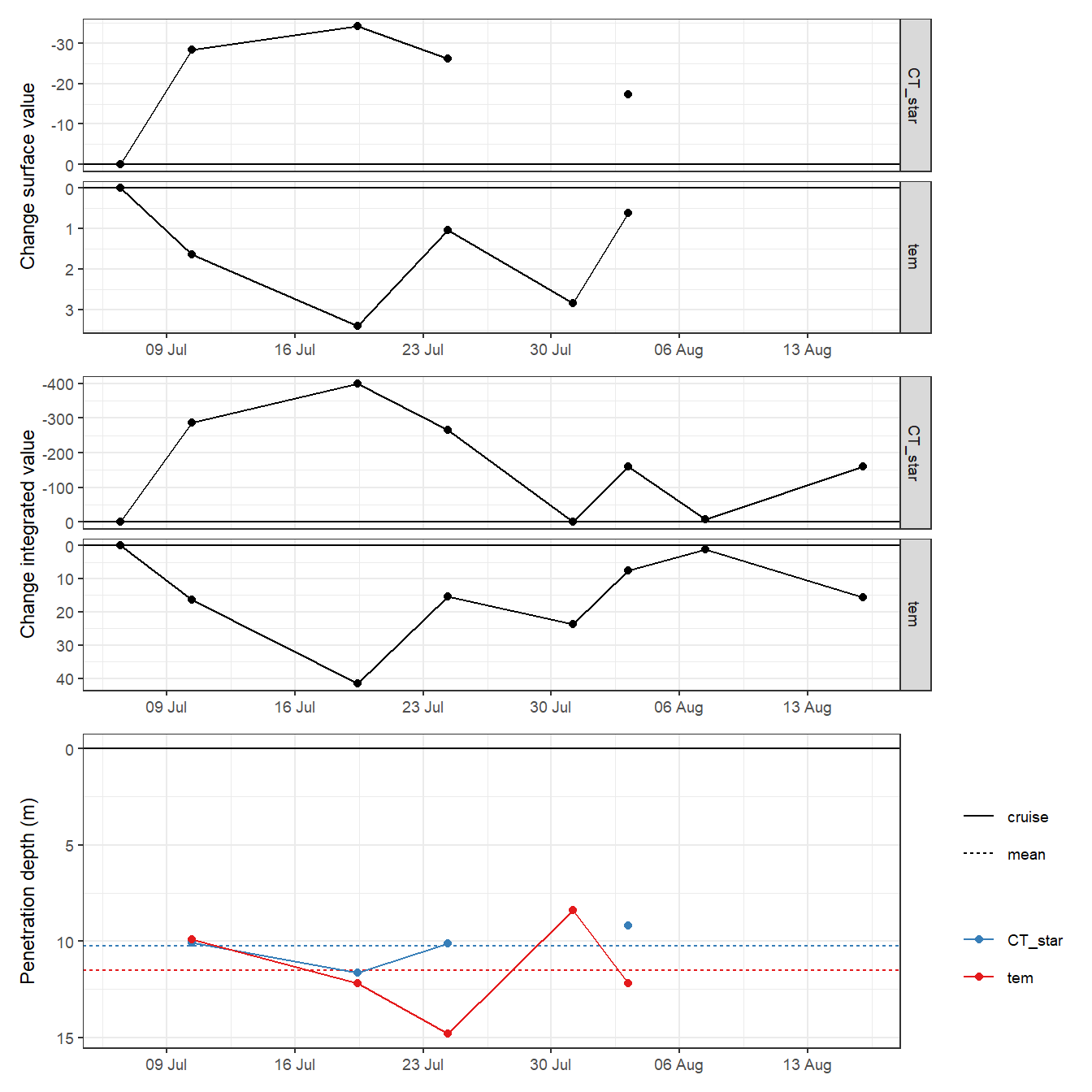

PD_mean

# A tibble: 2 x 3
  var     i_dep_mean i_dep_sd
  <chr>        <dbl>    <dbl>
1 CT_star       10.3     1.03
2 tem           11.5     2.46

rm(p_surface, p_integrated, p_pen_dep)
rm(PD, PD_mean, tm_profiles_ID_long)

3 GETM model

3.1 Read netcdf file

# read netcdf file
nc <- 
  nc_open(here::here("data/input/GETM", "Finnmaid.E.3d.2018.nc"))

# extract latitude vector
lat <- ncvar_get(nc, "latc")

# extract start time
time_start <- nc$dim$time$units %>%
  substr(start = 15, stop = 33) %>%
  ymd_hms()

# create time vecotr
t <- time_start + ncvar_get(nc, "time")
rm(time_start)

# extract depths vector
d <- ncvar_get(nc, "zax")

# read model data
for (var_3d in c("salt", "temp")) {
  
  # store the data in a 3-dimensional array
  array <-
    ncvar_get(nc, var_3d) 
  
  # find NA value
  fillvalue <- ncatt_get(nc, var_3d, "_FillValue")
  
  # replace NA value with NA
  array[array == fillvalue$value] <- NA
  
  for (i in seq(1, length(t), 1)) {
    # i <- 3
    array_slice <- array[, , i] # slices data from one day
    
    # convert to tibble
    array_slice_df <- as.data.frame(t(array_slice))
    array_slice_df <- as_tibble(array_slice_df)
    
    # rename, format and subset data
    gt_3d_part <- array_slice_df %>%
      set_names(as.character(lat)) %>%
      mutate(dep = -d) %>%
      gather("lat", "value", 1:length(lat)) %>%
      mutate(lat = as.numeric(lat)) %>%
      filter(
        lat > parameters$getm_low_lat,
        lat < parameters$getm_high_lat,
        dep <= parameters$max_dep
      ) %>%
      mutate(var = var_3d,
             date_time = t[i]) %>%
      select(date_time, dep, value, var)
    
    
    if (exists("gt_3d")) {
      gt_3d <- bind_rows(gt_3d, gt_3d_part)
    } else {
      gt_3d <- gt_3d_part
    }
    
    rm(array_slice, array_slice_df, gt_3d_part)
    
  }
  rm(array, fillvalue)
  
}

nc_close(nc)
rm(nc)

# subset time period
# calculate daily, regional mean profile in study area
gt_3d_long <- gt_3d %>%
  filter(date_time >= parameters$getm_start_date &
           date_time <= parameters$getm_end_date) %>%
  group_by(date_time, var, dep) %>%
  summarise_all(list(value =  ~ mean(., na.rm = TRUE))) %>% # regional averaging
  ungroup()

gt_3d <- gt_3d_long %>%
  pivot_wider(values_from = value, names_from = var) %>%
  rename(sal = salt, tem = temp)


rm(i, lat, d, t, var_3d)

3.2 Sal and tem profiles

gt_3d_long %>%
  ggplot(aes(value, dep,
             col = date_time,
             group = date_time)) +
  geom_path() +
  scale_y_reverse(expand = c(0, 0)) +
  scale_color_viridis_c(name = "Date", trans = "time") +
  facet_wrap( ~ var, scales = "free_x", ncol = 2)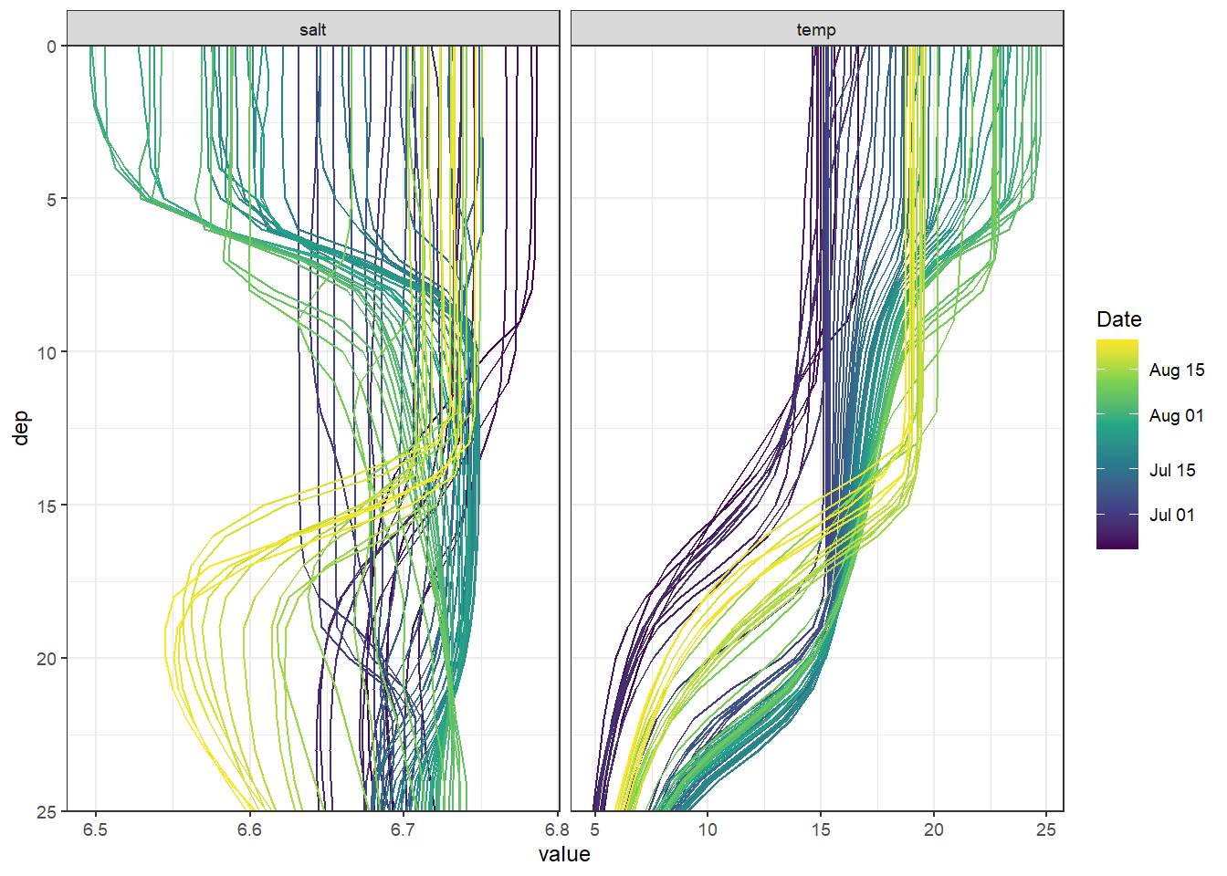

rm(gt_3d_long)

3.3 Comparison BloomSail

Vertical, 1m-gridded BloomSail CTD profiles were used for comparison with GETM results. Note that the sampling location does not match exactly.

3.3.1 Interpolate GETM to BloomSail

GETM results were linearly interpolated to the BloomSail depth levels and the mean cruise dates.

gt_3d_int <- gt_3d %>%
  mutate(dep_int = dep + 0.5) %>%
  group_by(date_time) %>%
  mutate(sal_int = approxfun(dep, sal)(dep_int),
         tem_int = approxfun(dep, tem)(dep_int)) %>%
  ungroup() %>%
  select(date_time,
         dep = dep_int,
         sal = sal_int,
         tem = tem_int) %>%
  drop_na()

rm(gt_3d)

# join GETM and BloomSail profiles
tm_gt_3d <- full_join(
  gt_3d_int,
  tm_profiles_ID %>% select(date_time = date_time_ID,
                            dep, sal, tem),
  by = c("date_time", "dep"),
  suffix = c("_gt", "_tm")
)

# calculate density profiles
tm_gt_3d <- tm_gt_3d  %>%
  mutate(
    rho_gt = swSigma(
      salinity = sal_gt,
      temperature = tem_gt,
      pressure = dep / 10
    ),
    rho_tm = swSigma(
      salinity = sal_tm,
      temperature = tem_tm,
      pressure = dep / 10
    )
  )

# interpolate to BloomSail time stamp
tm_gt_3d <- tm_gt_3d %>%
  arrange(date_time) %>%
  group_by(dep) %>%
  mutate(
    tem_gt = approxfun(date_time, tem_gt)(date_time),
    sal_gt = approxfun(date_time, sal_gt)(date_time),
    rho_gt = approxfun(date_time, rho_gt)(date_time)
  ) %>%
  ungroup() %>%
  drop_na()

3.3.2 S, T, rho profiles

# convert to long format
tm_gt_3d_long <- tm_gt_3d %>%
  pivot_longer(
    sal_gt:rho_tm,
    values_to = "value",
    names_to = c("var", "source"),
    names_sep = "_"
  )

tm_gt_3d_long %>%
  ggplot(aes(value, dep,
             col = date_time,
             group = date_time)) +
  geom_path() +
  scale_y_reverse(expand = c(0, 0), name = "Depth (m)") +
  scale_color_viridis_c(name = "Date", trans = "time") +
  facet_grid(source ~ var, scales = "free_x")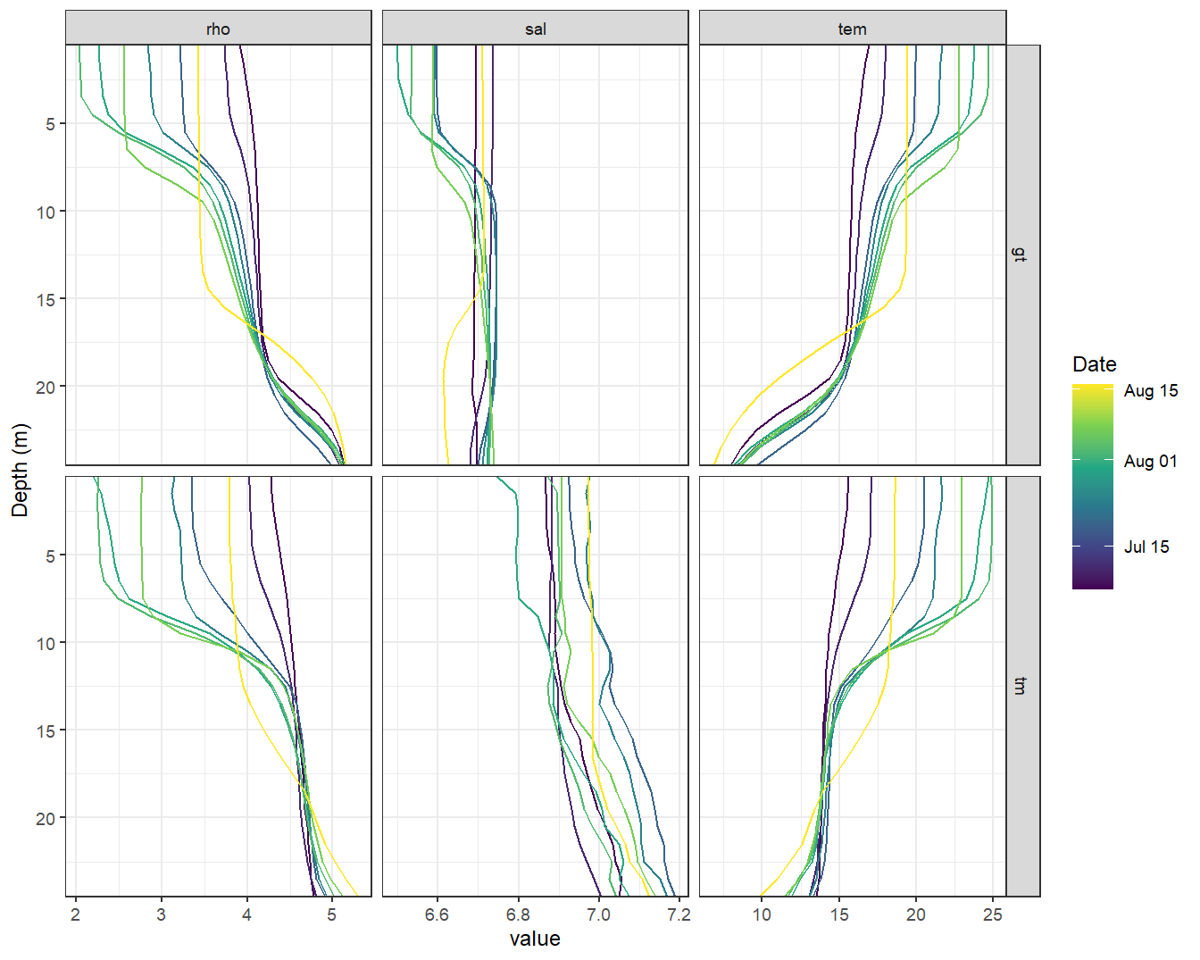

STD profiles modeled with GETM (upper panels, gt) and measured during BloomSail campaign (lower panels, ts)

3.3.3 S, T, rho offset profiles

tm_gt_3d <- tm_gt_3d_long %>%
  pivot_wider(values_from = "value", names_from = "source") %>%
  mutate(value_diff = gt - tm)

tm_gt_3d %>%
  ggplot(aes(value_diff, dep,
             col = date_time,
             group = date_time)) +
  geom_vline(xintercept = 0, col = "red") +
  geom_path() +
  scale_y_reverse(expand = c(0, 0), name = "Depth (m)") +
  scale_color_viridis_c(name = "Date", trans = "time") +
  facet_grid(. ~ var, scales = "free_x") +
  labs(x = "Difference GETM (gt) - Bloomsail (ts)")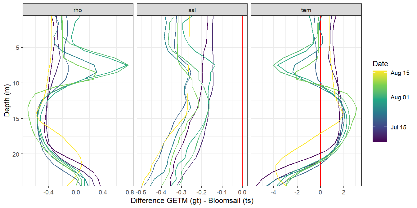

Offset STD profiles comparing modeled with GETM (upper panels, gt) and measured during BloomSail campaign (lower panels, ts)

rm(tm_gt_3d, tm_gt_3d_long)

4 SOOP Finnmaid

4.1 Data preparation

fm <-
 read_csv(here::here("data/intermediate/_summarized_data_files",
                      "fm_bloomsail.csv"))

fm <- fm %>% 
  filter(date_time > parameters$getm_start_date,
         date_time < parameters$getm_end_date) %>% 
  select(ID, date_time, sensor, sal, tem, pCO2) %>% 
  mutate(ID = as.factor(ID))

4.1.1 C_T* calculation

Calculate C_T* based on fixed A_T and salinity mean values.

# read mean bottle data
fixed_values <- 
  read_csv(here::here("data/intermediate/_summarized_data_files", "tb_fix.csv"))

# calculate CT*
fm <- fm %>%
  mutate(
    CT_star = carb(
      24,
      var1 = pCO2,
      var2 = fixed_values$AT * 1e-6,
      S = fixed_values$sal,
      T = tem,
      k1k2 = "m10",
      kf = "dg",
      ks = "d",
      gas = "insitu"
    )[, 16] * 1e6
  )

4.1.2 Regional averaging

Calculate regional mean and sd values for each crossing of the area.

fm_ID <- fm %>%
  pivot_longer(c(pCO2, sal, tem, CT_star),
               values_to = "value",
               names_to = "var") %>%
  group_by(ID) %>%
  mutate(date_time_ID = mean(date_time)) %>%
  ungroup() %>%
  select(-date_time) %>%
  group_by(ID, date_time_ID, sensor, var) %>%
  summarise_all(list( ~ mean(.), ~ sd(.)), na.rm = TRUE) %>%
  ungroup() %>%
  rename(value = mean)

4.1.3 Read tm profile data

Read original profile data and calculate surface mean and sd values.

tm_profiles <-
  read_csv(
    here::here(
      "data/intermediate/_merged_data_files/NCP_best_guess",
      "tm_profiles.csv"
    )
  )

# surface mean calculation
tm_profiles_ID_long_surface <- tm_profiles %>%
  filter(dep < parameters$surface_dep) %>%
  select(-c(dep, date_ID, station, date_time, lat, lon, pCO2_corr)) %>%
  mutate(ID = as.factor(ID)) %>%
  pivot_longer(sal:CT_star, values_to = "value", names_to = "var") %>%
  group_by(ID, date_time_ID, var) %>%
  summarise_all(list( ~ mean(.), ~ sd(.)), na.rm = TRUE) %>%
  ungroup()

4.1.4 Timeseries

fm_ID %>%
  ggplot() +
  geom_rect(data = fixed_values,
            aes(
              xmin = start,
              xmax = end,
              ymin = -Inf,
              ymax = Inf
            ),
            alpha = 0.2) +
  geom_path(aes(x = date_time_ID, y = value)) +
  geom_ribbon(aes(
    x = date_time_ID,
    y = value,
    ymax = value + sd,
    ymin = value - sd,
    fill = "Finnmaid"
  ),
  alpha = 0.3) +
  geom_ribbon(
    data = tm_profiles_ID_long_surface,
    aes(
      x = date_time_ID,
      ymin = mean - sd,
      ymax = mean + sd,
      fill = "BloomSail"
    ),
    alpha = 0.3
  ) +
  geom_point(aes(x = date_time_ID, y = value, col = sensor)) +
  geom_point(data = tm_profiles_ID_long_surface,
             aes(x = date_time_ID, y = mean, col = "BloomSail")) +
  geom_line(data = tm_profiles_ID_long_surface,
            aes(x = date_time_ID, y = mean, col = "BloomSail")) +
  facet_grid(var ~ ., scales = "free_y") +
  scale_color_brewer(palette = "Set1") +
  scale_fill_brewer(palette = "Set1", name = "+/- SD") +
  scale_x_datetime(date_breaks = "week",
                   date_labels = "%b %d") +
  theme(axis.title.x = element_blank())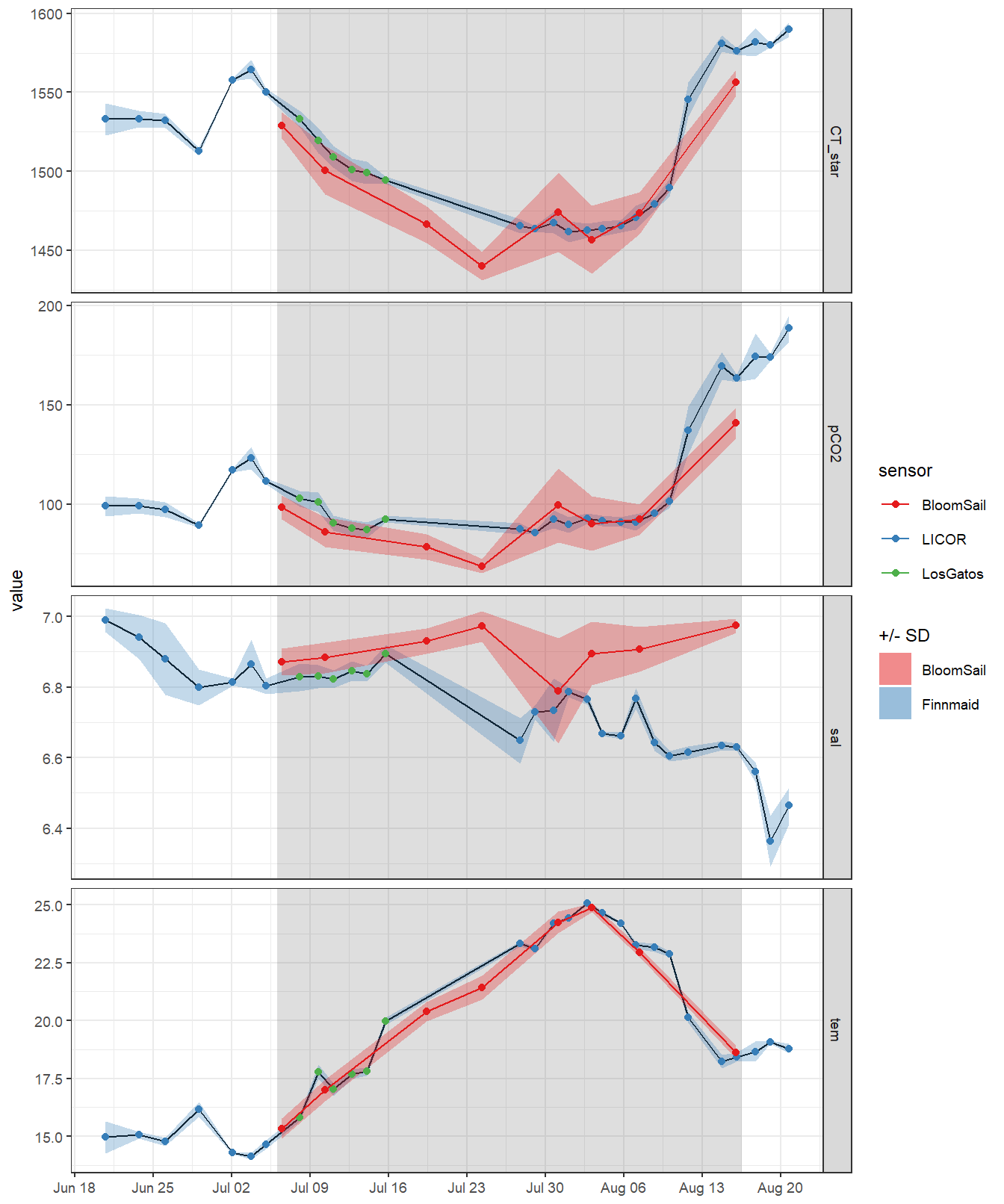

4.1.5 Missing observations

The observational gaps in the Finnmaid SST and C_T* time series were filled with:

two BloomSail observations
an interpolated Finnmaid value to match the starting date

The time series was restricted to the period where BloomSail observations are available.

# create data frame with start dates
tm_start_date <- tm_profiles_ID_long_surface %>% 
  filter(ID %in% c("180705"),
         var %in% c("tem", "CT_star")) %>% 
  select(date_time_ID, ID, var) %>% 
  mutate(sensor = "interpolated")

# add start dates to Finnmaid data
fm_tm_ID <- full_join(fm_ID, tm_start_date) %>% 
  arrange(date_time_ID) %>% 
  filter(var %in% c("tem", "CT_star"))

# interpolate Finnmaid to BloomSail start date
fm_tm_ID <- fm_tm_ID %>% 
  group_by(var) %>% 
  mutate(value = approxfun(date_time_ID, value)(date_time_ID)) %>% 
  ungroup()

rm(tm_start_date)

# subset BloomSail data in Finnmaid gap
tm_gap <- tm_profiles_ID_long_surface %>%
  filter(ID %in% c("180718", "180723"),
         var %in% c("tem", "CT_star")) %>%
  select(date_time_ID, ID, var, value = mean) %>%
  mutate(sensor = "BloomSail")

# add data to fill Finnmaid gap
fm_tm_ID <- full_join(fm_tm_ID, tm_gap) %>%
  arrange(date_time_ID) %>%
  select(-sd) %>%
  filter(var %in% c("tem", "CT_star")) %>%
  mutate(
    period = "BloomSail",
    period = if_else(date_time_ID < fixed_values$start, "pre-BloomSail", period),
    period = if_else(date_time_ID > fixed_values$end, "post-BloomSail", period)
  )

# filter only Finnmaid data within BloomSail period
fm_tm_ID <- fm_tm_ID %>%
  filter(period == "BloomSail") %>%
  select(-period)

rm(fm_ID, fm, tm_gap, tm_profiles_ID_long_surface, tm_profiles, fixed_values)

4.1.6 Final time series

fm_tm_ID %>%
  ggplot() +
  geom_path(aes(date_time_ID, value)) +
  geom_point(aes(date_time_ID, value, col = sensor)) +
  facet_grid(var ~ ., scales = "free_y") +
  scale_color_brewer(palette = "Set1") +
  scale_x_datetime(date_breaks = "week",
                   date_labels = "%b %d") +
  theme(axis.title.x = element_blank())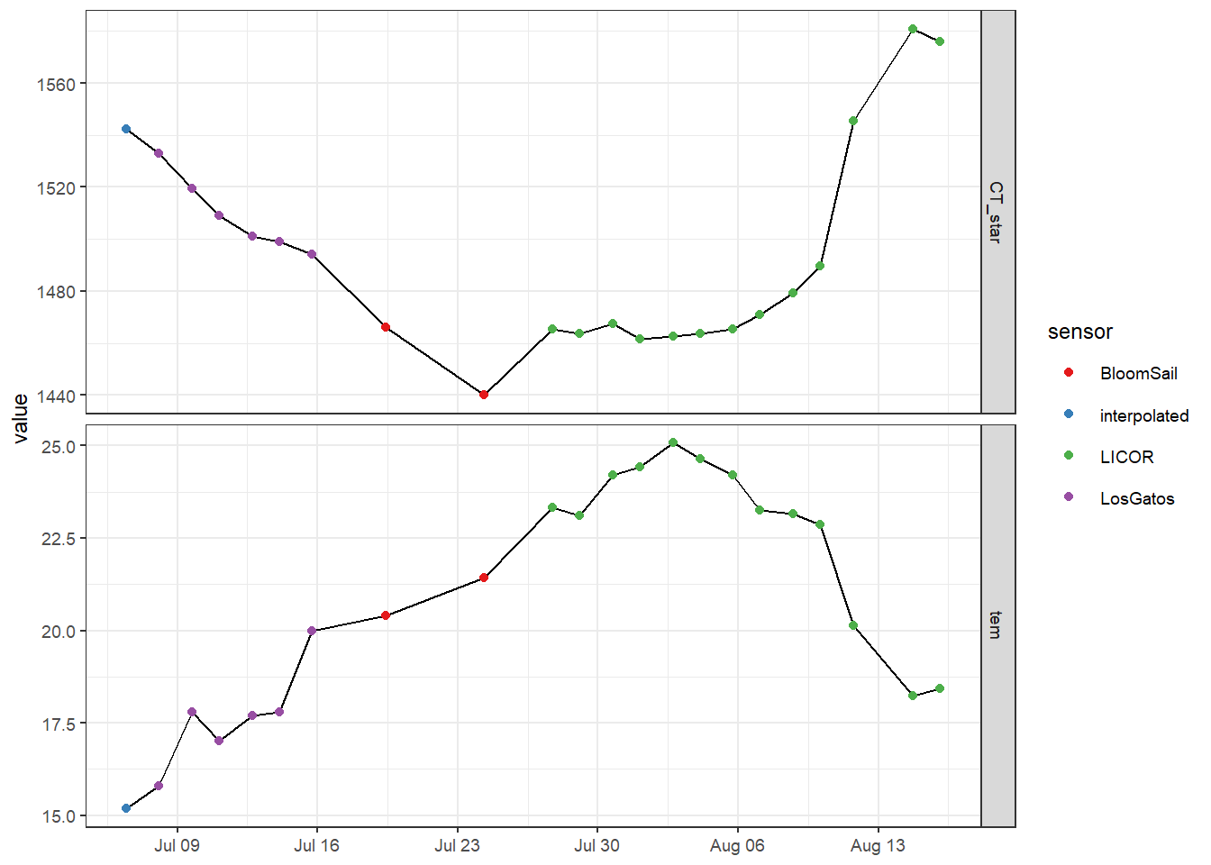

5 Merge all data sets

5.1 Merge fm and gt

# convert to wide format
fm_tm_ID_wide <- fm_tm_ID %>%
  filter(var %in% c("CT_star")) %>%
  select(date_time_ID, var, sensor, value) %>%
  pivot_wider(values_from = value, names_from = var)

# extend surface data with depth grid
fm_gt <- expand_grid(fm_tm_ID_wide, dep = unique(gt_3d_int$dep))

# join Finnmaid and GETM data
fm_gt <- full_join(fm_gt,
                   gt_3d_int %>% rename(date_time_ID = date_time)) %>%
  arrange(date_time_ID)

rm(fm_tm_ID_wide, fm_tm_ID, gt_3d_int)

5.2 Interpolate gt time stamp to fm

GETM data are interpolated to the time of Finnmaid observations.

fm_gt <- fm_gt %>%
  arrange(date_time_ID) %>%
  group_by(dep) %>%
  mutate(
    tem = approxfun(date_time_ID, tem)(date_time_ID),
    sal = approxfun(date_time_ID, sal)(date_time_ID)
  ) %>%
  ungroup() %>%
  arrange(dep) %>%
  filter(!is.na(CT_star))

5.3 Bind tm and fm_gt

Here, we merge the in-situ sensor data from SV Tina V with the Finnmaid+GETM data set, in order to perform following computations only once.

# subset relevant columns and assign source label
tm_profiles_ID <- tm_profiles_ID %>%
  select(-c(ID, pCO2)) %>%
  mutate(source = "tm",
         sensor = "BloomSail")

fm_gt <- fm_gt %>%
  mutate(source = "fm")

# Merge data sets
tm_fm_gt <- bind_rows(tm_profiles_ID, fm_gt)

rm(fm_gt, tm_profiles_ID)

5.4 Comparison

5.4.1 Surface time series

# convert to long format
tm_fm_gt_long <- tm_fm_gt %>%
  pivot_longer(sal:CT_star, values_to = "value", names_to = "var")

tm_fm_gt_long %>%
  filter(dep == 3.5) %>%
  ggplot(aes(date_time_ID, value, col = source)) +
  geom_path() +
  geom_point() +
  scale_x_datetime(date_breaks = "week",
                   date_labels = "%b %d") +
  facet_grid(var ~ ., scales = "free_y") +
  labs(title = "Time series at 3.5 m") +
  theme(axis.title.x = element_blank())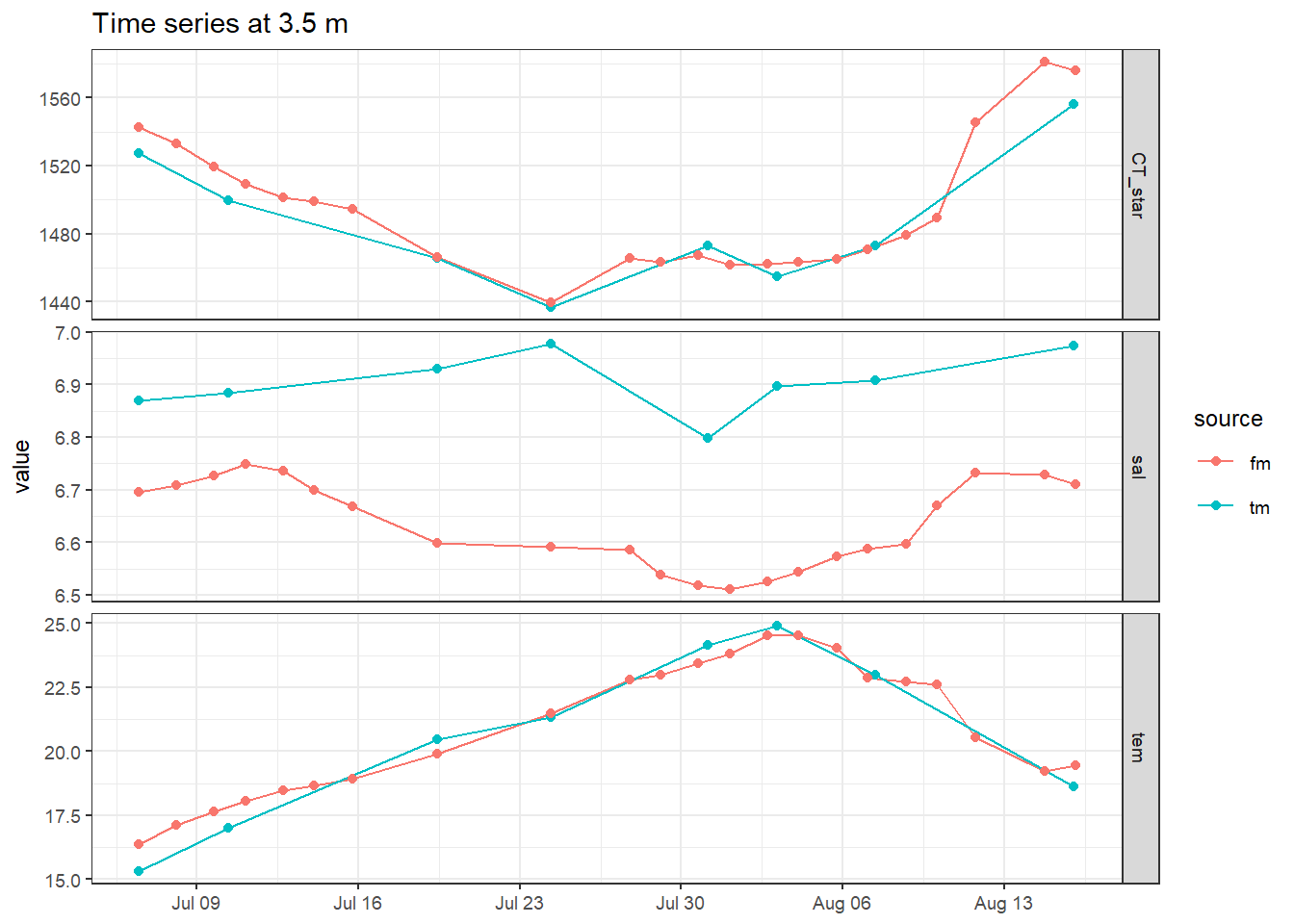

5.4.2 Hovmoeller temperature

bin <- 2

tm_fm_gt %>%
  ggplot(aes(date_time_ID, dep, z = tem)) +
  geom_contour_fill(breaks = MakeBreaks(bin)) +
  geom_vline(aes(xintercept = date_time_ID),
             col = "white",
             linetype = "1f") +
  scale_fill_viridis_c(
    name = "tem",
    option = "B",
    guide = "colorstrip",
    breaks = MakeBreaks(bin)
  ) +
  scale_y_reverse() +
  scale_x_datetime(date_breaks = "week",
                   date_labels = "%b %d") +
  coord_cartesian(expand = 0) +
  theme(axis.title.x = element_blank()) +
  facet_grid(source ~ .)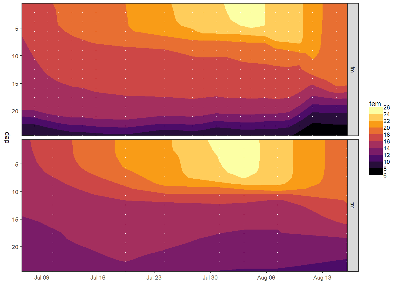

rm(bin)

6 Integration depths

6.1 MLD

6.1.1 Density calculation

tm_fm_gt <- tm_fm_gt %>%
  mutate(rho = swSigma(
    salinity = sal,
    temperature = tem,
    pressure = dep / 10
  ))

6.1.2 Hovmoeller density

bin <- 0.5

tm_fm_gt %>%
  ggplot() +
  geom_contour_fill(aes(date_time_ID, dep, z = rho),
                    breaks = MakeBreaks(bin)) +
  geom_vline(aes(xintercept = date_time_ID),
             col = "white",
             linetype = "1f") +
  scale_fill_viridis_c(
    name = "rho",
    option = "B",
    guide = "colorstrip",
    breaks = MakeBreaks(bin),
    direction = -1
  ) +
  scale_y_reverse() +
  scale_x_datetime(date_breaks = "week",
                   date_labels = "%b %d") +
  coord_cartesian(expand = 0) +
  theme(axis.title.x = element_blank()) +
  facet_grid(source ~ .)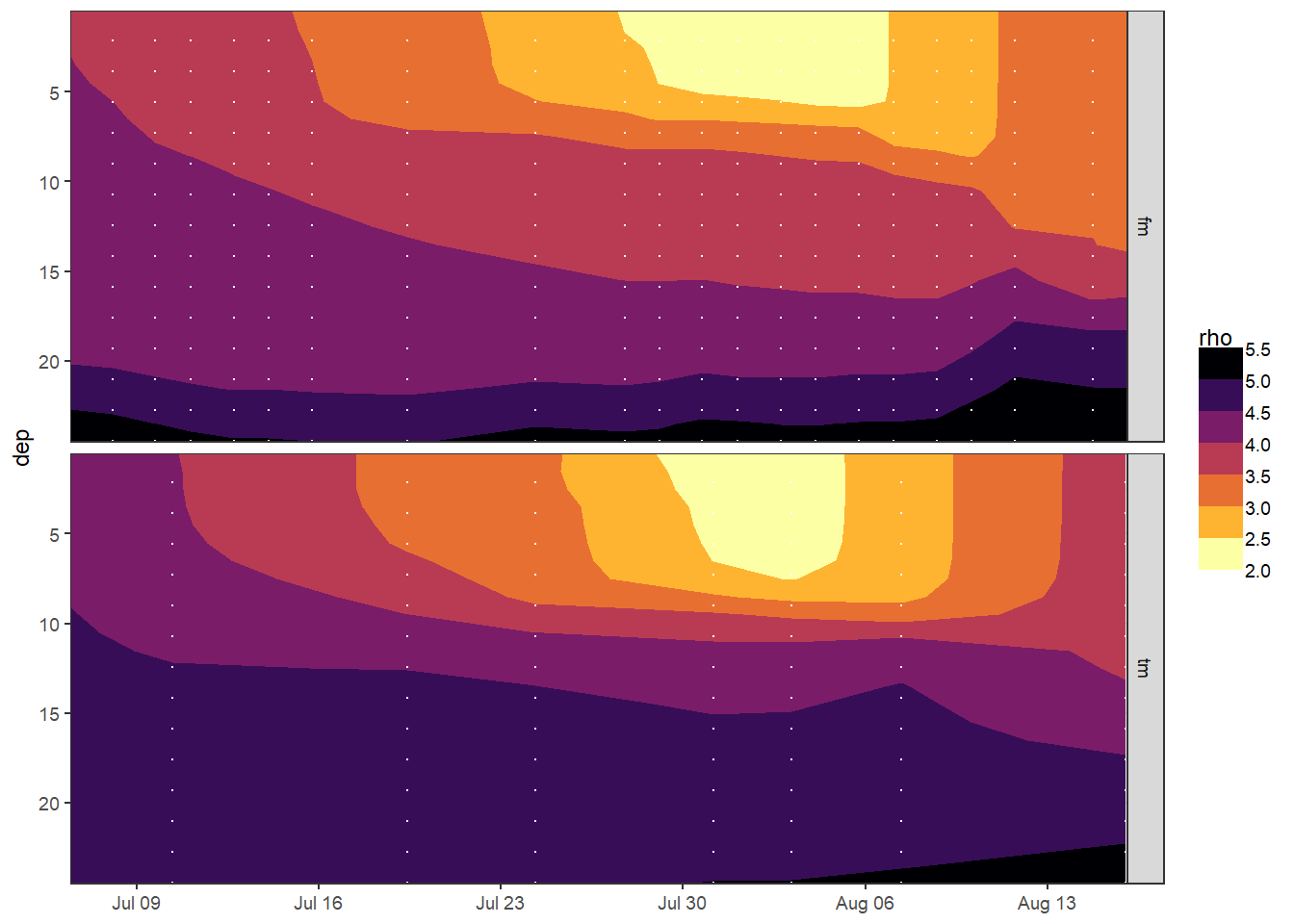

rm(bin)

6.1.3 MLD calculation

tm_fm_gt_MLD <- expand_grid(tm_fm_gt, rho_lim = parameters$rho_lim_integration_depths)

tm_fm_gt_MLD <- tm_fm_gt_MLD %>%
  arrange(dep) %>%
  group_by(date_time_ID, source, rho_lim) %>%
  mutate(d_rho = rho - first(rho)) %>%
  filter(d_rho > rho_lim) %>%
  summarise(MLD = min(dep)) %>%
  ungroup() %>%
  mutate(rho_lim = as.factor(rho_lim))

6.1.4 Hovmoeller MLD

bin <- 2

tm_fm_gt %>%
  ggplot() +
  geom_contour_fill(aes(date_time_ID, dep, z = tem),
                    breaks = MakeBreaks(bin)) +
  geom_path(data = tm_fm_gt_MLD, aes(date_time_ID, MLD, col = rho_lim)) +
  scale_fill_gradient(
    name = "Tem (°C)",
    guide = "colorstrip",
    breaks = MakeBreaks(bin),
    high = "grey80",
    low = "grey5"
  ) +
  scale_color_viridis_d() +
  scale_y_reverse() +
  scale_x_datetime(date_breaks = "week",
                   date_labels = "%b %d") +
  coord_cartesian(expand = 0) +
  labs(y = "Depth (m)") +
  theme(axis.title.x = element_blank()) +
  facet_grid(source ~ .)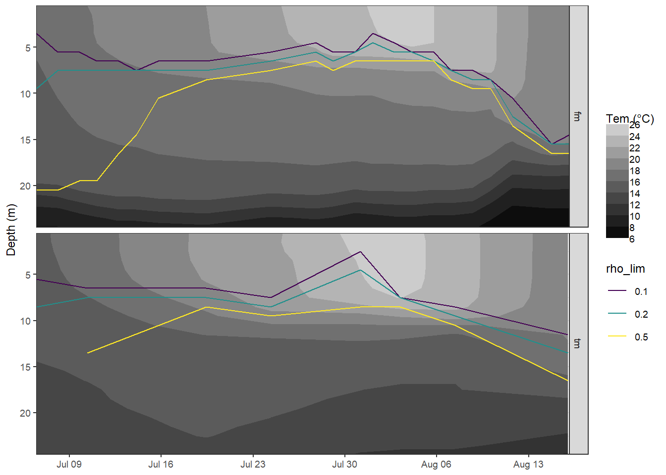

rm(bin)

6.1.5 Select rho criterion

MLD <- tm_fm_gt_MLD %>%
  filter(rho_lim == parameters$rho_lim) %>%
  select(-rho_lim) %>%
  rename(i_dep = MLD) %>%
  mutate(i_method = "MLD", i_res = "daily")

rm(tm_fm_gt_MLD)

6.1.6 Mean MLD

# Filter data before temperature peak, and calculate mean
MLD_mean <- MLD %>%
  filter(date_time_ID <= date_tem_max) %>%
  group_by(source) %>%
  summarise(MLD_mean = mean(i_dep, na.rm = TRUE),
            MLD_sd = sd(i_dep, na.rm = TRUE)) %>%
  ungroup()

MLD_mean

# A tibble: 2 x 3
  source MLD_mean MLD_sd
  <chr>     <dbl>  <dbl>
1 fm          5.5   1.18
2 tm          6     1.87

# format mean MLD data frame
MLD_mean <- MLD_mean %>%
  select(-MLD_sd) %>% 
  rename(i_dep = MLD_mean) %>%
  mutate(i_method = "MLD", i_res = "mean")

MLD_dates <- MLD %>%
  select(source, date_time_ID)

MLD_mean <- full_join(MLD_dates, MLD_mean)
MLD <- full_join(MLD, MLD_mean)

rm(MLD_mean)

6.2 TPD

6.2.1 Cumulative changes

tm_fm_gt_long <- tm_fm_gt %>%
  select(-c(sal)) %>%
  pivot_longer(c("tem", "CT_star"),
               values_to = "value",
               names_to = "var") %>%
  group_by(source, var, dep) %>%
  arrange(date_time_ID) %>%
  mutate(
    date_time_ID_diff = as.numeric(date_time_ID - lag(date_time_ID)),
    value_diff = value - lag(value, default = first(value)),
    value_diff_daily = value_diff / date_time_ID_diff,
    value_cum = cumsum(value_diff)
  ) %>%
  ungroup()

# select only temperature data
tm_fm_gt_long <- tm_fm_gt_long %>%
  filter(var == "tem") %>%
  select(-var)

6.2.2 Temperature profiles

Please note that the cumulative temperature profile of GETM shows a deep maximum below 20m, which must be attributed to water mass exchange rather than surface warming to radiation or heat uptake, which we want to capture here. Therefore, the integration depth of the GETM data was manually restricted to 19m.

tm_fm_gt_long %>%
  filter(date_time_ID == date_CT_min) %>%
  arrange(dep) %>%
  ggplot(aes(value_cum, dep)) +
  geom_vline(xintercept = 0) +
  geom_hline(yintercept = parameters$getm_i_dep) +
  geom_point() +
  geom_path() +
  scale_y_reverse() +
  labs(x = "Cumulative tem change",
       title = as.Date(date_CT_min)) +
  theme(legend.position = "left") +
  facet_grid(. ~ source, scales = "free_x")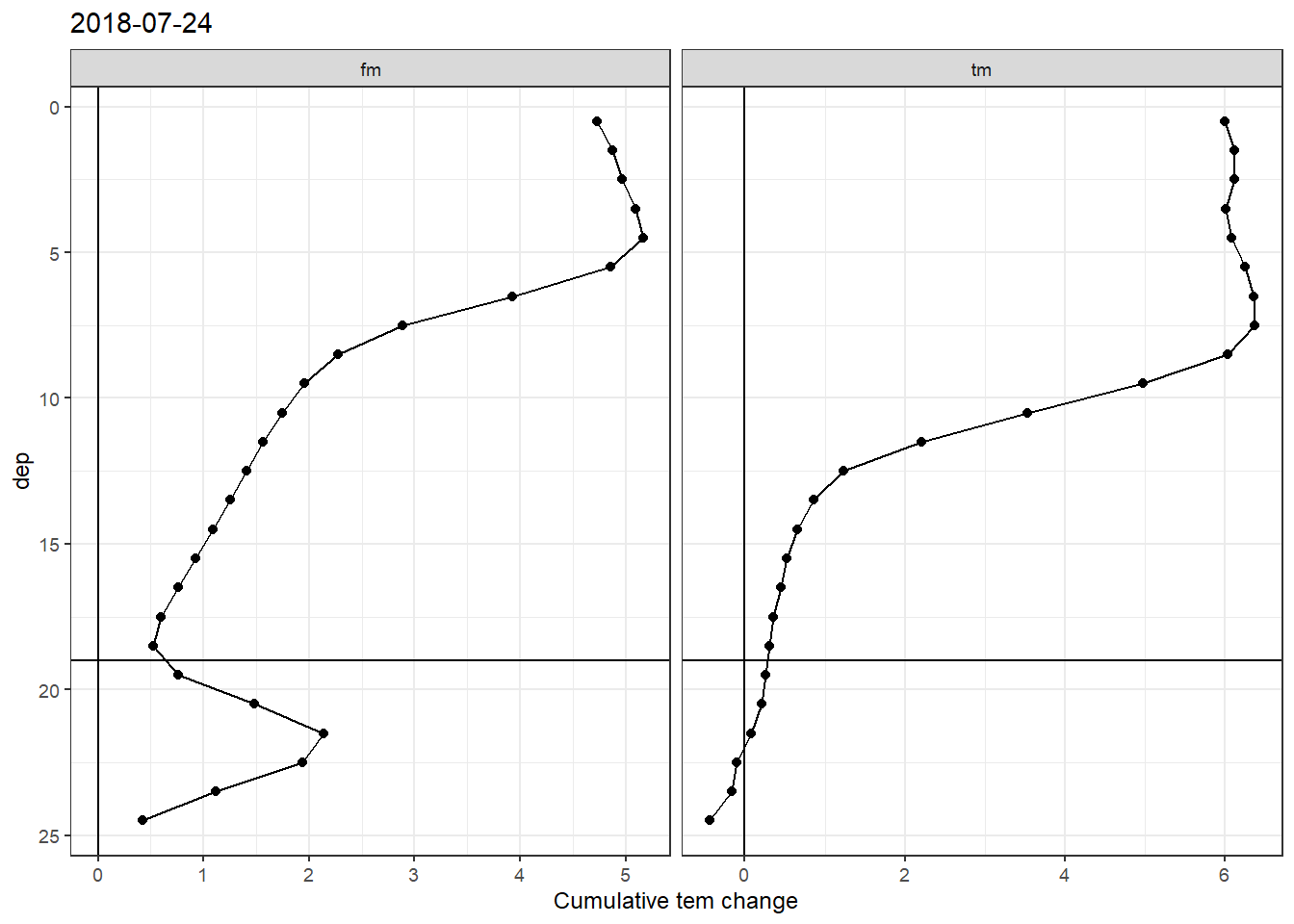

Profiles of cumulative temperature changes from the GETM model (label fm) and as measured in the field (label tm).

6.2.3 Cumulative TPD

# subset data at CT* minimum
tm_fm_gt_long_day <- tm_fm_gt_long %>%
  filter(date_time_ID == date_CT_min) %>%
  mutate(
    value_cum = if_else(value_cum < 0,
                        NaN, value_cum),
    value_cum = if_else(source == "fm" &
                          dep > parameters$getm_i_dep,
                        NaN, value_cum)
  )

# integrate cumulative changes
tm_fm_gt_long_day_dep <- tm_fm_gt_long_day %>%
  select(source, dep, value_cum) %>%
  group_by(source) %>%
  arrange(dep) %>%
  mutate(
    value_cum_i = sum(value_cum, na.rm = TRUE),
    value_cum_dep = cumsum(value_cum),
    value_cum_i_rel = value_cum_dep / value_cum_i * 100
  ) %>%
  ungroup()

# extract integrated cumulative value
value_cum <- tm_fm_gt_long_day_dep %>%
  group_by(source) %>%
  summarise(value_cum_i = mean(value_cum_i)) %>%
  ungroup()

# extract surface cumulative value
value_surface <- tm_fm_gt_long_day %>%
  select(source, dep, value_cum) %>%
  filter(dep < parameters$surface_dep) %>%
  group_by(source) %>%
  summarise(value_surface = mean(value_cum)) %>%
  ungroup()

# calculate TPD
TPD <- full_join(value_cum, value_surface)
TPD <- TPD %>%
  mutate(i_dep = value_cum_i / value_surface)

rm(value_cum, value_surface)

p_tm_fm_gt_long <- tm_fm_gt_long_day %>%
  arrange(dep) %>%
  ggplot(aes(value_cum, dep)) +
  geom_hline(aes(yintercept = parameters$i_dep_lim, col = "fixed\nintegration\ndepth")) +
  geom_hline(data = TPD, aes(yintercept = i_dep, col = "TPD\nestimate")) +
  geom_vline(xintercept = 0) +
  geom_point() +
  geom_path() +
  scale_y_reverse() +
  scale_color_brewer(palette = "Dark2", guide = FALSE) +
  labs(x = "Cumulative change") +
  theme(legend.position = "left") +
  facet_wrap(. ~ source, ncol = 1, scales = "free_x")

p_tm_fm_gt_long_rel <- tm_fm_gt_long_day_dep %>%
  ggplot(aes(value_cum_i_rel, dep)) +
  geom_hline(aes(yintercept = parameters$i_dep_lim, col = "fixed\nintegration\ndepth")) +
  geom_hline(data = TPD, aes(yintercept = i_dep, col = "TPD\nestimate")) +
  geom_vline(xintercept = 90) +
  geom_point() +
  geom_line() +
  scale_y_reverse(limits = c(25, 0)) +
  scale_color_brewer(palette = "Dark2", name = "") +
  scale_x_continuous(limits = c(0, NA)) +
  labs(x = "Relative contribution (%)") +
  facet_wrap(. ~ source, ncol = 1, scales = "free_x") +
  theme(axis.title.y = element_blank())

p_tm_fm_gt_long + p_tm_fm_gt_long_rel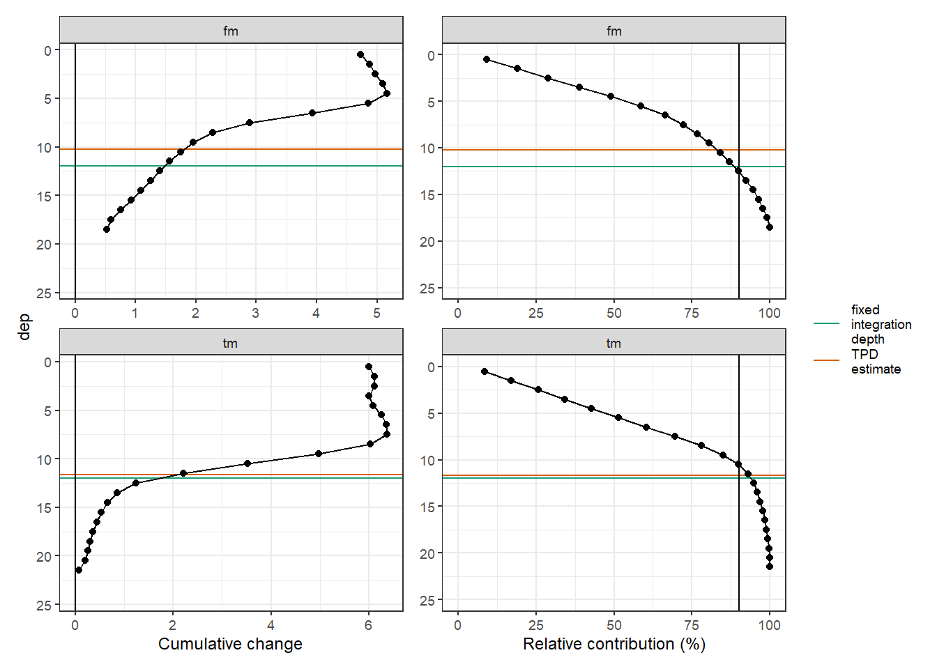

rm(
  tm_fm_gt_long_day,
  tm_fm_gt_long_day_dep,
  p_tm_fm_gt_long,
  p_tm_fm_gt_long_rel
)

TPD_cum <- TPD

rm(TPD)

6.2.4 Incremental TPD

# incremental changes of surface values
diff_surface <- tm_fm_gt_long %>%
  filter(dep < parameters$surface_dep) %>%
  group_by(date_time_ID, source) %>%
  summarise(value_diff_surface = mean(value_diff, na.rm = TRUE)) %>%
  ungroup() %>%
  mutate(value_diff_surface = if_else(value_diff_surface < 0,
                                      NaN, value_diff_surface))

tm_fm_gt_long <- full_join(tm_fm_gt_long, diff_surface)
rm(diff_surface)

# calculate penetration depths
TPD <- tm_fm_gt_long %>%
  mutate(
    value_diff = if_else(value_diff < 0,
                         NaN, value_diff),
    value_diff = if_else(source == "fm" & dep > 19,
                         NaN, value_diff)
  ) %>%
  group_by(date_time_ID, source) %>%
  summarise(
    value_diff_int = sum(value_diff, na.rm = TRUE),
    value_diff_surface = mean(value_diff_surface, na.rm = TRUE)
  ) %>%
  ungroup() %>%
  mutate(i_dep = value_diff_int / value_diff_surface)

# calculate mean TPD across bloom period
TPD_mean <- TPD %>%
  filter(date_time_ID <= date_CT_min) %>%
  group_by(source) %>%
  summarise(i_dep_sd = sd(i_dep, na.rm = TRUE),
            i_dep = mean(i_dep, na.rm = TRUE)) %>%
  ungroup()

p_surface <- TPD %>%
  ggplot(aes(date_time_ID, value_diff_surface, col = source)) +
  geom_hline(yintercept = 0) +
  geom_line() +
  geom_point() +
  scale_y_reverse(name = "Change surface value") +
  scale_x_datetime(breaks = "week", date_labels = "%d %b") +
  scale_color_brewer(palette = "Set1", direction = -1) +
  theme(axis.title.x = element_blank(),
        legend.title = element_blank())

p_integrated <- TPD %>%
  ggplot(aes(date_time_ID, value_diff_int, col = source)) +
  geom_hline(yintercept = 0) +
  geom_line() +
  geom_point() +
  scale_y_reverse(name = "Change integrated value") +
  scale_x_datetime(breaks = "week", date_labels = "%d %b") +
  scale_color_brewer(palette = "Set1", direction = -1) +
  theme(axis.title.x = element_blank(),
        legend.title = element_blank())

p_TPD <- TPD %>%
  ggplot(aes(date_time_ID, i_dep, col = source)) +
  geom_hline(yintercept = 0) +
  geom_hline(data = TPD_mean,
             aes(
               yintercept = i_dep,
               col = source,
               linetype = "mean"
             )) +
  geom_line(aes(linetype = "cruise")) +
  geom_point() +
  scale_y_reverse(name = "Penetration depth (m)", breaks = seq(0, 20, 5)) +
  scale_x_datetime(breaks = "week", date_labels = "%d %b") +
  scale_color_brewer(palette = "Set1", direction = -1) +
  theme(axis.title.x = element_blank(),
        legend.title = element_blank())


p_surface + p_integrated + p_TPD +
  plot_layout(ncol = 1)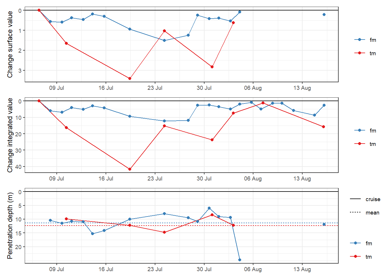

TPD_mean

# A tibble: 2 x 3
  source i_dep_sd i_dep
  <chr>     <dbl> <dbl>
1 fm         2.31  11.4
2 tm         2.46  12.3

rm(p_surface, p_integrated, p_TPD)

6.2.5 Join TPD estimates

TPD <- TPD %>%
  select(date_time_ID, source, i_dep) %>%
  mutate(i_method = "TPD", i_res = "daily") %>%
  filter(date_time_ID < date_tem_max) %>%
  mutate(i_dep = if_else(is.na(i_dep), 0, i_dep))

TPD_cum <- TPD_cum %>%
  select(source, i_dep) %>%
  mutate(i_method = "TPD", i_res = "cumulative")

TPD_cum <- full_join(MLD_dates, TPD_cum)

TPD_mean <- TPD_mean %>%
  select(source, i_dep) %>%
  mutate(i_method = "TPD", i_res = "mean")

TPD_mean <- full_join(MLD_dates, TPD_mean)

TPD <- full_join(TPD, TPD_cum)
TPD <- full_join(TPD, TPD_mean)

rm(TPD_cum, TPD_mean)

6.3 Join TPD and MLD

i_dep <- full_join(MLD, TPD)
rm(MLD, TPD)

6.4 Hovmoeller + MLD/TPD

bin <- 2

# prepare data sets
i_dep <- i_dep %>%
  mutate(source = factor(source, c("tm", "fm"))) %>%
  mutate(source = fct_recode(
    source,
    `SOOP Finnmaid + GETM model` = "fm",
    `SV Tina V (surface only)` = "tm"
  ))

tm_fm_gt <- tm_fm_gt %>%
  mutate(source = factor(source, c("tm", "fm"))) %>%
  mutate(source = fct_recode(
    source,
    `SOOP Finnmaid + GETM model` = "fm",
    `SV Tina V (surface only)` = "tm"
  ))

p_hov_dep <-
  tm_fm_gt %>%
  ggplot() +
  geom_contour_fill(aes(date_time_ID, dep, z = tem),
                    breaks = MakeBreaks(bin),
                    col = "black",
                    size = 0.1) +
  geom_path(data = i_dep %>% filter(i_res == "daily" & i_dep != 0),
            aes(date_time_ID, i_dep, col = i_method)) +
  scale_fill_gradient(
    name = "Temperature\n(\u00B0C)",
    guide = "colorstrip",
    breaks = MakeBreaks(bin),
    high = "grey90",
    low = "grey20"
  ) +
  guides(fill = guide_colorsteps(barheight = unit(35, "mm"),
                                 barwidth = unit(4, "mm"),
                                 frame.colour = "black",
                                 ticks = TRUE,
                                 ticks.colour = "black")) +
  scale_color_discrete(name = "Reconstruction", guide = FALSE) +
  scale_y_reverse() +
  scale_x_datetime(date_breaks = "week",
                   date_labels = "%b %d") +
  coord_cartesian(expand = 0) +
  labs(y = expression(atop(Depth, (m)))) +
  theme(
    axis.title.x = element_blank(),
    axis.text.x = element_blank(),
    axis.ticks.x = element_blank(),
    strip.background = element_blank(),
    strip.text.x = element_blank(),
    plot.margin = margin(0, 0, 0, 0, "cm")
  ) +
  facet_wrap( ~ source)

p_hov_dep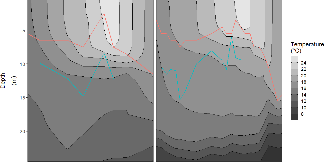

rm(bin)

7 Surface data + integr. depth

Here, we restrict all C_T* observations to surface waters, and merge with the integrations depth estimates.

# calculate surface water time series
tm_fm_gt_surface <- tm_fm_gt %>%
  filter(dep < parameters$surface_dep) %>%
  select(source, date_time_ID, sensor, CT_star) %>%
  group_by(source, date_time_ID, sensor) %>%
  summarise(CT_star = mean(CT_star, na.rm = TRUE)) %>%
  ungroup()

# calculate incremental and cumulative changes
tm_fm_gt_surface <- tm_fm_gt_surface %>%
  group_by(source) %>%
  arrange(date_time_ID) %>%
  mutate(
    date_time_ID_diff = as.numeric(date_time_ID - lag(date_time_ID)),
    CT_star_diff = CT_star - lag(CT_star, default = first(CT_star)),
    CT_star_cum = cumsum(CT_star_diff)
  ) %>%
  ungroup()

iCT <- full_join(tm_fm_gt_surface, i_dep)
rm(tm_fm_gt_surface)

8 NCP reconstruction

8.1 Integration of C_T*

Incremental depth-integrated changes of C_T* are calculated as the product of incremental changes of surface C_T* and the integration depth parameter.

# integrate incremental CT* changes across depth
iCT <- iCT %>% 
  mutate(CT_i_diff = CT_star_diff * i_dep)

# calculate cumulative changes
iCT <- iCT %>% 
  group_by(source, i_method, i_res) %>%
  arrange(date_time_ID) %>%
  mutate(CT_star_i_cum = cumsum(CT_i_diff/1000)) %>% 
  ungroup()

8.2 Read best-guess NCP

tm_NCP_cum <- read_csv(here::here("data/intermediate/_merged_data_files/NCP_best_guess",
                                  "tm_NCP_cum.csv"))

8.3 Adapt air sea flux

The air-sea fluxes of CO₂ previously calculated for the NCP best-guess were also applied to all reconstructed estimates

# prepare air sea flux data from best-guess approach
tm_NCP_cum_flux <- tm_NCP_cum %>%
  select(date_time, flux_cum)

tm_NCP_cum_flux <-
  expand_grid(
    tm_NCP_cum_flux,
    source = unique(iCT$source),
    i_method = unique(iCT$i_method),
    i_res = unique(iCT$i_res)
  )

NCP_flux <- full_join(iCT %>% rename(date_time = date_time_ID),
                      tm_NCP_cum_flux) %>%
  arrange(date_time)

# linear interpolation of cumulative changes to frequency of the flux estimates estimates
NCP_flux_int <- NCP_flux %>%
  filter(!(i_method == "MLD" & i_res == "cumulative")) %>%
  group_by(source, i_method, i_res) %>%
  mutate(
    CT_star_i_cum = approxfun(date_time, CT_star_i_cum)(date_time),
    flux_cum = approxfun(date_time, flux_cum)(date_time)
  ) %>%
  fill(flux_cum) %>%
  mutate(CT_star_i_flux_cum = CT_star_i_cum + flux_cum) %>%
  ungroup()

8.4 Time series

8.4.1 Without mixing corrrection

Below, we compare all derived NCP reconstructions to the best-guess time series of integrated C_T* changes, which were only corrected for air-sea fluxes but not for mixing.

iCT <- iCT %>%
  mutate(sensor = if_else(sensor == "BloomSail", sensor, "VOS"))

p_CT_star <- iCT %>%
  ggplot() +
  geom_path(aes(date_time_ID, CT_star)) +
  geom_point(aes(date_time_ID, CT_star, fill = sensor), shape = 21) +
  scale_fill_manual(values = c("white", "black"),
                    guide = FALSE) +
  scale_x_datetime(breaks = "week",
                   date_labels = "%d %b",
                   expand = c(0, 0)) +
  facet_wrap( ~ source) +
  labs(y = expression(atop(paste(C[T], "*"), (mu * mol ~ kg ^ {
    -1
  })))) +
  theme(
    axis.title.x = element_blank(),
    axis.text.x = element_blank(),
    axis.ticks.x = element_blank(),
    plot.margin = margin(0, 0, 0, 0, "cm"),
    panel.grid.minor = element_blank()
  )

p_iCT <- iCT %>%
  ggplot() +
  geom_hline(yintercept = 0) +
  geom_path(data = tm_NCP_cum,
            aes(date_time, CT_star_i_cum),
            col = "black") +
  geom_path(aes(
    date_time_ID,
    CT_star_i_cum,
    col = i_method,
    linetype = i_res
  )) +
  scale_color_discrete(name = "Reconstruction") +
  scale_x_datetime(
    breaks = "week",
    date_labels = "%d %b",
    sec.axis = dup_axis(),
    expand = c(0, 0)
  ) +
  scale_linetype(name = "Resolution") +
  facet_wrap(~ source) +
  labs(y = expression(atop(Integrated ~ nC[T], (mol ~ m ^ {
    -2
  })))) +
  guides(color = guide_legend(order = 1)) +
  theme(
    axis.title.x = element_blank(),
    strip.background = element_blank(),
    strip.text.x = element_blank(),
    axis.text.x.top = element_blank()
  )

p_CT_star / p_hov_dep / p_iCT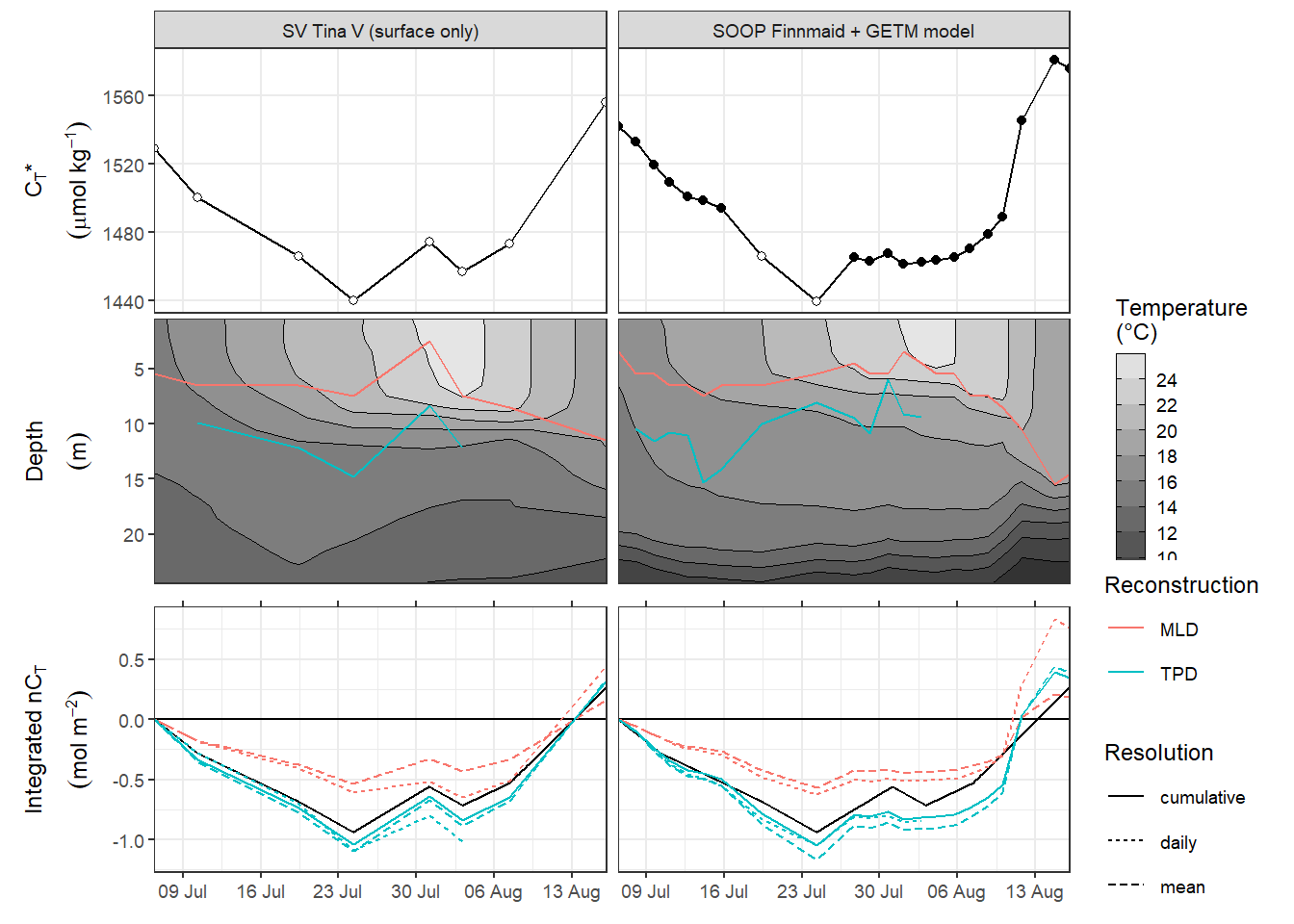

8.4.2 With mixing corrrection

Below, we compare four NCP reconstructions based on daily incremental integration depth estimates to the best-guess NCP time series, ie the integrated C_T* changes, which were corrected for air-sea fluxes and for mixing.

NCP_flux <- NCP_flux %>%
  mutate(i_res = factor(i_res, c("mean", "cumulative", "daily")))

p_NCP <- NCP_flux_int %>%
  filter(i_res %in% c("daily")) %>%
  ggplot() +
  geom_hline(yintercept = 0) +
  geom_path(
    data = tm_NCP_cum,
    aes(date_time, CT_star_i_flux_mix_cum, linetype = "best \U2013 guess"),
    col = "black"
  ) +
  geom_path(aes(
    date_time,
    CT_star_i_flux_cum,
    col = i_method,
    linetype = "reconstruction"
  )) +
  scale_color_discrete(name = "Integration depth") +
  scale_x_datetime(
    breaks = "week",
    date_labels = "%d %b",
    expand = c(0, 0)
  ) +
  scale_linetype_manual(name = "NCP estimate",
                        values = c(2, 1)) +
  facet_wrap(~ source) +
  labs(y = expression(atop(-~NCP, (mol ~ m ^ {
    -2
  })))) +
  guides(color = guide_legend(order = 1)) +
  theme(
    axis.title.x = element_blank(),
    strip.background = element_blank(),
    strip.text.x = element_blank(),
    plot.margin = margin(0, 0, 0, 0, "cm"),
    panel.grid.minor = element_blank()
  )

p_CT_star / p_hov_dep / p_NCP +
  plot_annotation(tag_levels = 'a')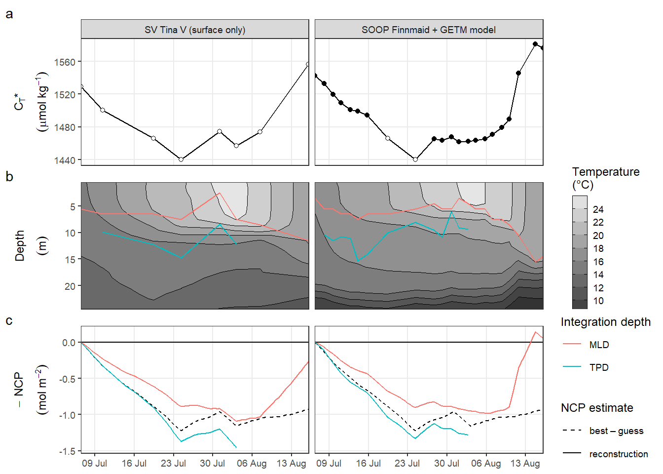

ggsave(
  here::here("output/Plots/Figures_publication/article",
             "Fig_6.pdf"),
  width = 160,
  height = 155,
  dpi = 300,
  units = "mm"
)

ggsave(
  here::here("output/Plots/Figures_publication/article",
             "Fig_6.png"),
  width = 160,
  height = 155,
  dpi = 300,
  units = "mm"
)

sessionInfo()

R version 4.0.3 (2020-10-10)
Platform: x86_64-w64-mingw32/x64 (64-bit)
Running under: Windows 10 x64 (build 19042)

Matrix products: default

locale:
[1] LC_COLLATE=English_Germany.1252  LC_CTYPE=English_Germany.1252   
[3] LC_MONETARY=English_Germany.1252 LC_NUMERIC=C                    
[5] LC_TIME=English_Germany.1252    

attached base packages:
[1] stats     graphics  grDevices utils     datasets  methods   base     

other attached packages:
 [1] metR_0.9.0        lubridate_1.7.9.2 patchwork_1.1.1   seacarb_3.2.14   
 [5] oce_1.2-0         gsw_1.0-5         testthat_3.0.1    ncdf4_1.17       
 [9] forcats_0.5.0     stringr_1.4.0     dplyr_1.0.2       purrr_0.3.4      
[13] readr_1.4.0       tidyr_1.1.2       tibble_3.0.4      ggplot2_3.3.3    
[17] tidyverse_1.3.0   workflowr_1.6.2  

loaded via a namespace (and not attached):
 [1] httr_1.4.2         jsonlite_1.7.2     viridisLite_0.3.0  here_1.0.1        
 [5] modelr_0.1.8       assertthat_0.2.1   highr_0.8          cellranger_1.1.0  
 [9] yaml_2.2.1         pillar_1.4.7       backports_1.2.1    glue_1.4.2        
[13] digest_0.6.27      RColorBrewer_1.1-2 promises_1.1.1     checkmate_2.0.0   
[17] rvest_0.3.6        colorspace_2.0-0   plyr_1.8.6         htmltools_0.5.0   
[21] httpuv_1.5.4       pkgconfig_2.0.3    broom_0.7.5        haven_2.3.1       
[25] scales_1.1.1       whisker_0.4        later_1.1.0.1      git2r_0.27.1      
[29] generics_0.1.0     farver_2.0.3       ellipsis_0.3.1     withr_2.3.0       
[33] cli_2.2.0          magrittr_2.0.1     crayon_1.3.4       readxl_1.3.1      
[37] evaluate_0.14      ps_1.5.0           fs_1.5.0           fansi_0.4.1       
[41] xml2_1.3.2         tools_4.0.3        data.table_1.13.6  hms_0.5.3         
[45] lifecycle_0.2.0    munsell_0.5.0      reprex_0.3.0       isoband_0.2.3     
[49] compiler_4.0.3     rlang_0.4.10       grid_4.0.3         rstudioapi_0.13   
[53] labeling_0.4.2     rmarkdown_2.6      gtable_0.3.0       DBI_1.1.0         
[57] R6_2.5.0           knitr_1.30         utf8_1.1.4         rprojroot_2.0.2   
[61] stringi_1.5.3      Rcpp_1.0.5         vctrs_0.3.6        dbplyr_2.0.0      
[65] tidyselect_1.1.0   xfun_0.19

NCP reconstruction

Jens Daniel Müller

18 May, 2021