NIES-ML3_GCB

workflowr

• Summary
• Checks
• Past versions

Last updated: 2025-03-06

Checks: 7 0

Knit directory: heatwave_co2_flux_2023/analysis/

This reproducible R Markdown analysis was created with workflowr (version 1.7.1). The Checks tab describes the reproducibility checks that were applied when the results were created. The Past versions tab lists the development history.

---

R Markdown file: up-to-date

Great! Since the R Markdown file has been committed to the Git repository, you know the exact version of the code that produced these results.

Environment: empty

Great job! The global environment was empty. Objects defined in the global environment can affect the analysis in your R Markdown file in unknown ways. For reproduciblity it’s best to always run the code in an empty environment.

Seed: set.seed(20240307)

The command set.seed(20240307) was run prior to running the code in the R Markdown file. Setting a seed ensures that any results that rely on randomness, e.g. subsampling or permutations, are reproducible.

Session information: recorded

Great job! Recording the operating system, R version, and package versions is critical for reproducibility.

Cache: none

Nice! There were no cached chunks for this analysis, so you can be confident that you successfully produced the results during this run.

File paths: relative

Great job! Using relative paths to the files within your workflowr project makes it easier to run your code on other machines.

Repository version: 8936cec

Great! You are using Git for version control. Tracking code development and connecting the code version to the results is critical for reproducibility.

The results in this page were generated with repository version 8936cec. See the Past versions tab to see a history of the changes made to the R Markdown and HTML files.

Note that you need to be careful to ensure that all relevant files for the analysis have been committed to Git prior to generating the results (you can use wflow_publish or wflow_git_commit). workflowr only checks the R Markdown file, but you know if there are other scripts or data files that it depends on. Below is the status of the Git repository when the results were generated:

Ignored files:
    Ignored:    .Rhistory
    Ignored:    .Rproj.user/
    Ignored:    data
    Ignored:    output/

Untracked files:
    Untracked:  analysis/CSIR-ML6_GCB.Rmd
    Untracked:  code/gas_flux_kwko.R

Unstaged changes:
    Modified:   analysis/_site.yml
    Modified:   analysis/child/pCO2_product_analysis.Rmd
    Modified:   analysis/child/pCO2_product_preprocessing.Rmd
    Modified:   analysis/child/pCO2_product_synopsis.Rmd
    Modified:   code/Workflowr_project_managment.R

Note that any generated files, e.g. HTML, png, CSS, etc., are not included in this status report because it is ok for generated content to have uncommitted changes.

---

These are the previous versions of the repository in which changes were made to the R Markdown (analysis/NIES-ML3_GCB.Rmd) and HTML (docs/NIES-ML3_GCB.html) files. If you’ve configured a remote Git repository (see ?wflow_git_remote), click on the hyperlinks in the table below to view the files as they were in that past version.

File	Version	Author	Date	Message
Rmd	8936cec	jens-daniel-mueller	2025-03-06	Include Watson product

---

center <- -160
boundary <- center + 180
target_crs <- paste0("+proj=robin +over +lon_0=", center)
# target_crs <- paste0("+proj=eqearth +over +lon_0=", center)
# target_crs <- paste0("+proj=eqearth +lon_0=", center)
# target_crs <- paste0("+proj=igh_o +lon_0=", center)

worldmap <- ne_countries(scale = 'small',
                         type = 'map_units',
                         returnclass = 'sf')

worldmap <- worldmap %>% st_break_antimeridian(lon_0 = center)
worldmap_trans <- st_transform(worldmap, crs = target_crs)

# ggplot() +
#   geom_sf(data = worldmap_trans)

coastline <- ne_coastline(scale = 'small', returnclass = "sf")
coastline <- st_break_antimeridian(coastline, lon_0 = 200)
coastline_trans <- st_transform(coastline, crs = target_crs)

# ggplot() +
#   geom_sf(data = worldmap_trans, fill = "grey", col="grey") +
#   geom_sf(data = coastline_trans)


bbox <- st_bbox(c(xmin = -180, xmax = 180, ymax = 65, ymin = -78), crs = st_crs(4326))
bbox <- st_as_sfc(bbox)
bbox_trans <- st_break_antimeridian(bbox, lon_0 = center)

bbox_graticules <- st_graticule(
  x = bbox_trans,
  crs = st_crs(bbox_trans),
  datum = st_crs(bbox_trans),
  lon = c(20, 20.001),
  lat = c(-78,65),
  ndiscr = 1e3,
  margin = 0.001
)

bbox_graticules_trans <- st_transform(bbox_graticules, crs = target_crs)
rm(worldmap, coastline, bbox, bbox_trans)

# ggplot() +
#   geom_sf(data = worldmap_trans, fill = "grey", col="grey") +
#   geom_sf(data = coastline_trans) +
#   geom_sf(data = bbox_graticules_trans)

lat_lim <- ext(bbox_graticules_trans)[c(3,4)]*1.002
lon_lim <- ext(bbox_graticules_trans)[c(1,2)]*1.005

# ggplot() +
#   geom_sf(data = worldmap_trans, fill = "grey90", col = "grey90") +
#   geom_sf(data = coastline_trans) +
#   geom_sf(data = bbox_graticules_trans, linewidth = 1) +
#   coord_sf(crs = target_crs,
#            ylim = lat_lim,
#            xlim = lon_lim,
#            expand = FALSE) +
#   theme(
#     panel.border = element_blank(),
#     axis.text = element_blank(),
#     axis.ticks = element_blank()
#   )

latitude_graticules <- st_graticule(
  x = bbox_graticules,
  crs = st_crs(bbox_graticules),
  datum = st_crs(bbox_graticules),
  lon = c(20, 20.001),
  lat = c(-60,-30,0,30,60),
  ndiscr = 1e3,
  margin = 0.001
)

latitude_graticules_trans <- st_transform(latitude_graticules, crs = target_crs)

latitude_labels <- data.frame(lat_label = c("60°N","30°N","Eq.","30°S","60°S"),
                 lat = c(60,30,0,-30,-60)-4, lon = c(35)-c(0,2,4,2,0))

latitude_labels <- st_as_sf(x = latitude_labels,
               coords = c("lon", "lat"),
               crs = "+proj=longlat")

latitude_labels_trans <- st_transform(latitude_labels, crs = target_crs)

# ggplot() +
#   geom_sf(data = worldmap_trans, fill = "grey", col = "grey") +
#   geom_sf(data = coastline_trans) +
#   geom_sf(data = bbox_graticules_trans) +
#   geom_sf(data = latitude_graticules_trans,
#           col = "grey60",
#           linewidth = 0.2) +
#   geom_sf_text(data = latitude_labels_trans,
#                aes(label = lat_label),
#                size = 3,
#                col = "grey60")

Read data

path_pCO2_products <-
  "/nfs/kryo/work/datasets/gridded/ocean/2d/observation/pco2/gcb_2024_pco2_products/"

library(ncdf4)
nc <-
  nc_open(paste0(
    path_pCO2_products,
    "GCB-2024_dataprod_NIES-ML3_1982-2023.nc"
  ))

print(nc)

pco2_product <-
  read_ncdf(
    paste0(
      path_pCO2_products,
      "GCB-2024_dataprod_NIES-ML3_1982-2023.nc"
    ),
    var = c("fco2atm", "fgco2", "kw", "alpha", "sfco2", "tos"),
    ignore_bounds = TRUE,
    make_units = FALSE
  )

pco2_product <- pco2_product %>%
  as_tibble()

pco2_product <- pco2_product %>%
  drop_na()

pco2_product <-
  pco2_product %>%
  rename(temperature = tos,
         atm_fco2 = fco2atm,
         sol = alpha)

pco2_product <-
  pco2_product %>%
  mutate(area = earth_surf(lat, lon),
         year = year(time),
         month = month(time))

pco2_product <-
  pco2_product %>% 
  mutate(lon = if_else(lon < 20, lon + 360, lon))

pco2_product <-
  pco2_product %>%
  mutate(dfco2 = sfco2 - atm_fco2)

pco2_product <-
  pco2_product %>% 
  mutate(fgco2 = -fgco2 * 60 * 60 * 24 * 365,
         kw_sol = kw * sol * 1e-2 * 24 * 365)

pco2_product <-
  pco2_product %>%
  select(-c(kw, sol))

pCO2_product_preprocessing <-
  knitr::knit_expand(
    file = here::here("analysis/child/pCO2_product_preprocessing.Rmd"),
    product_name = "NIES-ML3_GCB"
  )

Preprocessing

# model <- TRUE
model <- str_detect('NIES-ML3_GCB', "FESOM-REcoM|ETHZ-CESM")

Load masks

biome_mask <-
  read_rds(here::here("data/biome_mask.rds"))

region_mask <-
  read_rds(here::here("data/region_mask.rds"))

map <-
  read_rds(here::here("data/map.rds"))

key_biomes <-
  read_rds(here::here("data/key_biomes.rds"))

Define labels and breaks

labels_breaks <- function(i_name) {
  
  if (i_name == "dco2") {
    i_legend_title <- "ΔpCO<sub>2</sub><br>(µatm)"
  }
  
  if (i_name == "dfco2") {
    i_legend_title <- "ΔfCO<sub>2</sub><br>(µatm)"
  }
  
  if (i_name == "atm_co2") {
    i_legend_title <- "pCO<sub>2,atm</sub><br>(µatm)"
  }
  
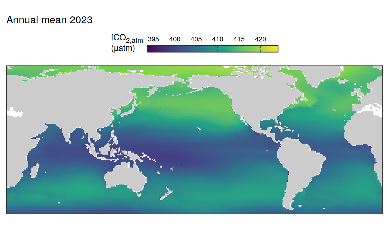
  if (i_name == "atm_fco2") {
    i_legend_title <- "fCO<sub>2,atm</sub><br>(µatm)"
  }
  
  if (i_name == "sol") {
    i_legend_title <- "K<sub>0</sub><br>(mol m<sup>-3</sup> µatm<sup>-1</sup>)"
  }
  
  if (i_name == "kw") {
    i_legend_title <- "k<sub>w</sub><br>(m yr<sup>-1</sup>)"
  }
  
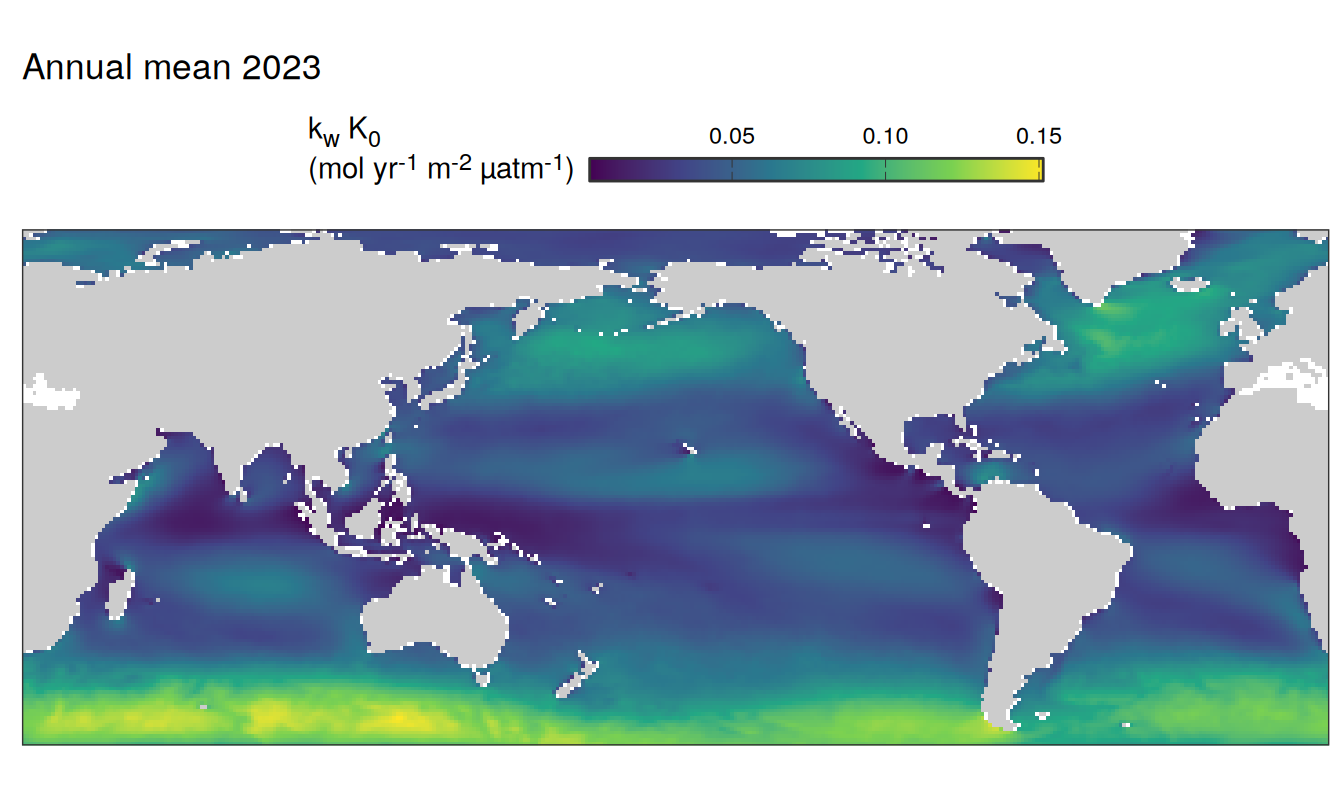
  if (i_name == "kw_sol") {
    i_legend_title <- "k<sub>w</sub> K<sub>0</sub><br>(mol yr<sup>-1</sup> m<sup>-2</sup> µatm<sup>-1</sup>)"
  }
  
  if (i_name == "spco2") {
    i_legend_title <- "pCO<sub>2,ocean</sub><br>(µatm)"
  }
  
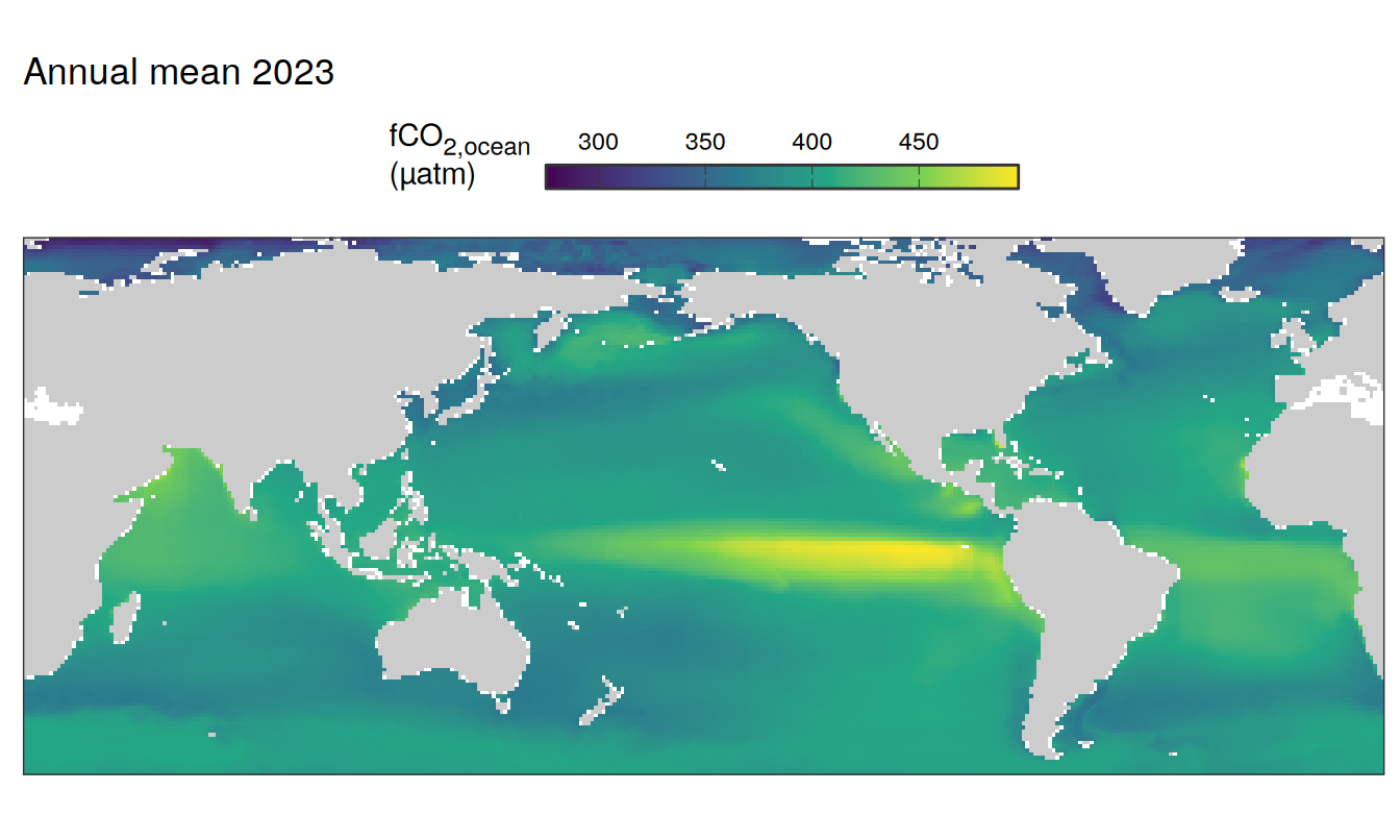
  if (i_name == "sfco2") {
    i_legend_title <- "fCO<sub>2,ocean</sub><br>(µatm)"
  }
  
  if (i_name == "intpp") {
    i_legend_title <- "NPP<sub>int</sub><br>(mol m<sup>-2</sup> yr<sup>-1</sup>)"
  }

  if (i_name == "no3") {
    i_legend_title <- "NO<sub>3</sub><br>(μmol kg<sup>-1</sup>)"
  }

  if (i_name == "o2") {
    i_legend_title <- "O<sub>2</sub><br>(μmol kg<sup>-1</sup>)"
  }

  if (i_name == "dissic") {
    i_legend_title <- "DIC<br>(μmol kg<sup>-1</sup>)"
  }

  if (i_name == "sdissic") {
    i_legend_title <- "sDIC<br>(μmol kg<sup>-1</sup>)"
  }

  if (i_name == "cstar") {
    i_legend_title <- "C*<br>(μmol kg<sup>-1</sup>)"
  }

  if (i_name == "talk") {
    i_legend_title <- "TA<br>(μmol kg<sup>-1</sup>)"
  }

  if (i_name == "stalk") {
    i_legend_title <- "sTA<br>(μmol kg<sup>-1</sup>)"
  }
  
  
  if (i_name == "sdissic_stalk") {
    i_legend_title <- "sDIC-sTA<br>(μmol kg<sup>-1</sup>)"
  }
  
  if (i_name == "sfco2_total") {
    i_legend_title <- "total"
  }
  
  if (i_name == "sfco2_therm") {
    i_legend_title <- "thermal"
  }
  
  if (i_name == "sfco2_nontherm") {
    i_legend_title <- "non-thermal"
  }
  
  if (i_name == "fgco2") {
    i_legend_title <- "FCO<sub>2</sub><br>(mol m<sup>-2</sup> yr<sup>-1</sup>)"
  }
  
  if (i_name == "fgco2_predict") {
    i_legend_title <- "FCO<sub>2</sub> pred.<br>(mol m<sup>-2</sup> yr<sup>-1</sup>)"
  }
  
  if (i_name == "fgco2_hov") {
    i_legend_title <- "FCO<sub>2</sub><br>(PgC deg<sup>-1</sup> yr<sup>-1</sup>)"
  }
  
  if (i_name == "fgco2_int") {
    i_legend_title <- "FCO<sub>2</sub><br>(PgC yr<sup>-1</sup>)"
  }
  
  if (i_name == "fgco2_predict_int") {
    i_legend_title <- "FCO<sub>2</sub> pred.<br>(PgC yr<sup>-1</sup>)"
  }
  
  if (i_name == "thetao") {
    i_legend_title <- "Temp.<br>(°C)"
  }
  
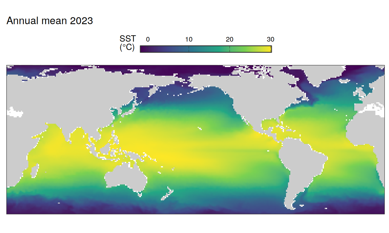
  if (i_name == "temperature") {
    i_legend_title <- "SST<br>(°C)"
  }
  
  if (i_name == "salinity") {
    i_legend_title <- "SSS"
  }
  
  if (i_name == "so") {
    i_legend_title <- "salinity"
  }
  
  if (i_name == "chl") {
    i_legend_title <- "lg(Chl-a)<br>(lg(mg m<sup>-3</sup>))"
  }
  
  if (i_name == "mld") {
    i_legend_title <- "MLD<br>(m)"
  }
  
  if (i_name == "press") {
    i_legend_title <- "pressure<sub>atm</sub><br>(Pa)"
  }
  
  if (i_name == "wind") {
    i_legend_title <- "Wind <br>(m sec<sup>-1</sup>)"
  }
  
  if (i_name == "SSH") {
    i_legend_title <- "SSH <br>(m)"
  }
  
  if (i_name == "fice") {
    i_legend_title <- "Sea ice <br>(%)"
  }
  
    
  if (i_name == "resid_fgco2") {
    i_legend_title <-
      "Observed"
  }
    
  if (i_name == "resid_fgco2_dfco2") {
    i_legend_title <-
      "ΔfCO<sub>2</sub>"
  }
    
  if (i_name == "resid_fgco2_kw_sol") {
    i_legend_title <-
      "k<sub>w</sub> K<sub>0</sub>"
  }
    
  if (i_name == "resid_fgco2_dfco2_kw_sol") {
    i_legend_title <-
      "k<sub>w</sub> K<sub>0</sub> X ΔfCO<sub>2</sub>"
  }
    
  if (i_name == "resid_fgco2_sum") {
    i_legend_title <-
      "∑"
  }
    
  if (i_name == "resid_fgco2_offset") {
    i_legend_title <-
      "Obs. - ∑"
  }
  
  all_labels_breaks <- lst(i_legend_title)
  
  return(all_labels_breaks)
  
}

x_axis_labels <-
  c(
    "dco2" = labels_breaks("dco2")$i_legend_title,
    "dfco2" = labels_breaks("dfco2")$i_legend_title,
    "atm_co2" = labels_breaks("atm_co2")$i_legend_title,
    "atm_fco2" = labels_breaks("atm_fco2")$i_legend_title,
    "sol" = labels_breaks("sol")$i_legend_title,
    "kw" = labels_breaks("kw")$i_legend_title,
    "kw_sol" = labels_breaks("kw_sol")$i_legend_title,
    "intpp" = labels_breaks("intpp")$i_legend_title,
    "no3" = labels_breaks("no3")$i_legend_title,
    "o2" = labels_breaks("o2")$i_legend_title,
    "dissic" = labels_breaks("dissic")$i_legend_title,
    "sdissic" = labels_breaks("sdissic")$i_legend_title,
    "cstar" = labels_breaks("cstar")$i_legend_title,
    "talk" = labels_breaks("talk")$i_legend_title,
    "stalk" = labels_breaks("stalk")$i_legend_title,
    "sdissic_stalk" = labels_breaks("sdissic_stalk")$i_legend_title,
    "spco2" = labels_breaks("spco2")$i_legend_title,
    "sfco2" = labels_breaks("sfco2")$i_legend_title,
    "sfco2_total" = labels_breaks("sfco2_total")$i_legend_title,
    "sfco2_therm" = labels_breaks("sfco2_therm")$i_legend_title,
    "sfco2_nontherm" = labels_breaks("sfco2_nontherm")$i_legend_title,
    "fgco2" = labels_breaks("fgco2")$i_legend_title,
    "fgco2_predict" = labels_breaks("fgco2_predict")$i_legend_title,
    "fgco2_hov" = labels_breaks("fgco2_hov")$i_legend_title,
    "fgco2_int" = labels_breaks("fgco2_int")$i_legend_title,
    "fgco2_predict_int" = labels_breaks("fgco2_int")$i_legend_title,
    "thetao" = labels_breaks("thetao")$i_legend_title,
    "temperature" = labels_breaks("temperature")$i_legend_title,
    "salinity" = labels_breaks("salinity")$i_legend_title,
    "so" = labels_breaks("so")$i_legend_title,
    "chl" = labels_breaks("chl")$i_legend_title,
    "mld" = labels_breaks("mld")$i_legend_title,
    "press" = labels_breaks("press")$i_legend_title,
    "wind" = labels_breaks("wind")$i_legend_title,
    "SSH" = labels_breaks("SSH")$i_legend_title,
    "fice" = labels_breaks("fice")$i_legend_title,
    "resid_fgco2" = labels_breaks("resid_fgco2")$i_legend_title,
    "resid_fgco2_dfco2" = labels_breaks("resid_fgco2_dfco2")$i_legend_title,
    "resid_fgco2_kw_sol" = labels_breaks("resid_fgco2_kw_sol")$i_legend_title,
    "resid_fgco2_dfco2_kw_sol" = labels_breaks("resid_fgco2_dfco2_kw_sol")$i_legend_title,
    "resid_fgco2_sum" = labels_breaks("resid_fgco2_sum")$i_legend_title,
    "resid_fgco2_offset" = labels_breaks("resid_fgco2_offset")$i_legend_title
  )

Analysis settings

name_quadratic_fit <- c("atm_co2", "atm_fco2", "spco2", "sfco2")
# name_quadratic_fit <- c(name_quadratic_fit, "dfco2", "fgco2", "fgco2_int", "temperature")

start_year <- 1990

name_divergent <- c("dco2", "dfco2", "fgco2", "fgco2_hov", "fgco2_int")

Data preprocessing

pco2_product <-
  pco2_product %>%
  filter(year >= start_year)

pco2_product_interior <-
  pco2_product_interior %>%
  filter(time >= ymd(paste0(start_year, "-01-01")))

biome_mask <- biome_mask %>% 
  mutate(area = earth_surf(lat, lon))

pco2_product <-
  full_join(pco2_product,
            biome_mask)

# set all values outside biome mask to NA

pco2_product <-
  pco2_product %>%
  mutate(across(-c(lat, lon, time, area, year, month, biome), 
                ~ if_else(is.na(biome), NA, .)))

Compuations

Maps

Biome means

pco2_product_biome_monthly_global <-
  pco2_product %>%
  filter(!is.na(fgco2)) %>%
  mutate(fgco2_int = fgco2) %>%
  mutate(biome = case_when(str_detect(biome, "SO-SPSS|SO-ICE|Arctic") ~ "Polar",
                           TRUE ~ "Global non-polar")) %>%
  filter(biome == "Global non-polar") %>%
  select(-c(lon, lat, year, month)) %>%
  group_by(time, biome) %>%
  summarise(across(-c(fgco2_int, area),
                   ~ weighted.mean(., area, na.rm = TRUE)),
            across(fgco2_int,
                   ~ sum(. * area, na.rm = TRUE) * 12.01 * 1e-15)) %>%
  ungroup()

pco2_product_biome_monthly_biome <-
  pco2_product %>%
  filter(!is.na(fgco2)) %>% 
  mutate(fgco2_int = fgco2) %>% 
  select(-c(lon, lat, year, month)) %>% 
  group_by(time, biome) %>%
  summarise(across(-c(fgco2_int, area),
                   ~ weighted.mean(., area, na.rm = TRUE)),
            across(fgco2_int,
                   ~ sum(. * area, na.rm = TRUE) * 12.01 * 1e-15)) %>%
  ungroup()


pco2_product_biome_monthly <-
  bind_rows(pco2_product_biome_monthly_global,
            pco2_product_biome_monthly_biome)

rm(
  pco2_product_biome_monthly_global,
  pco2_product_biome_monthly_biome
)


pco2_product_biome_monthly <-
  pco2_product_biome_monthly %>% 
  filter(!is.na(biome))

pco2_product_biome_monthly <-
  pco2_product_biome_monthly %>%
  mutate(year = year(time),
         month = month(time),
         .after = time)

pco2_product_biome_monthly <-
  pco2_product_biome_monthly %>%
  pivot_longer(-c(time, year, month, biome))


pco2_product_biome_annual <-
  pco2_product_biome_monthly %>%
  group_by(year, biome, name) %>%
  summarise(value = mean(value)) %>%
  ungroup()

Profiles

pco2_product_interior <- 
  left_join(
    biome_mask,
    pco2_product_interior
  )

pco2_product_profiles <- pco2_product_interior %>%
  fselect(-c(lat, lon)) %>%
  fgroup_by(biome, depth, time) %>% {
    add_vars(fgroup_vars(., "unique"),
             fmean(.,
                   w = area,
                   keep.w = FALSE,
                   keep.group_vars = FALSE))
  }

pco2_product_profiles <-
  pco2_product_profiles %>%
  mutate(
    year = year(time),
    month = month(time)
  )

gc()

Zonal mean sections

pco2_product_interior <- 
  left_join(
    region_mask,
    pco2_product_interior %>% select(-c(biome, area))
  )

pco2_product_zonal_mean <- pco2_product_interior %>%
  fselect(-c(lon)) %>%
  fgroup_by(region, depth, lat, time) %>% {
    add_vars(fgroup_vars(., "unique"),
             fmean(.,
                   keep.group_vars = FALSE))
  }

pco2_product_zonal_mean <-
  pco2_product_zonal_mean %>%
  mutate(
    year = year(time),
    month = month(time)
  )

gc()

rm(pco2_product_interior)
gc()

Absolute values

Hovmoeller plots

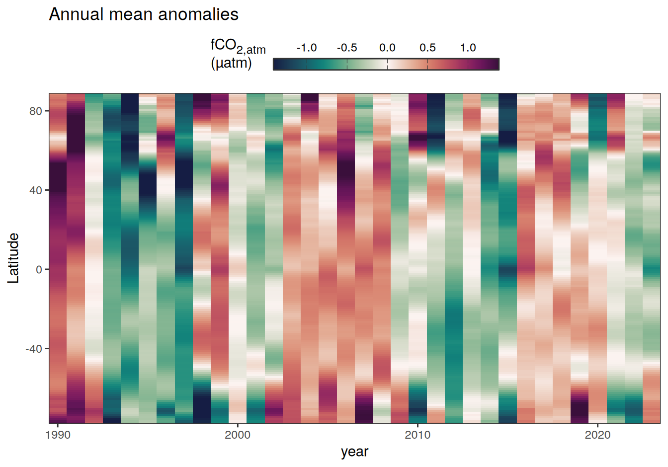
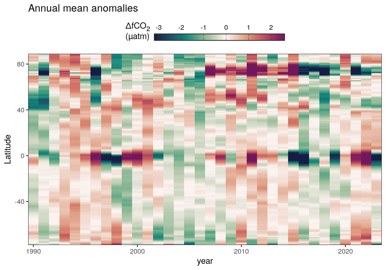
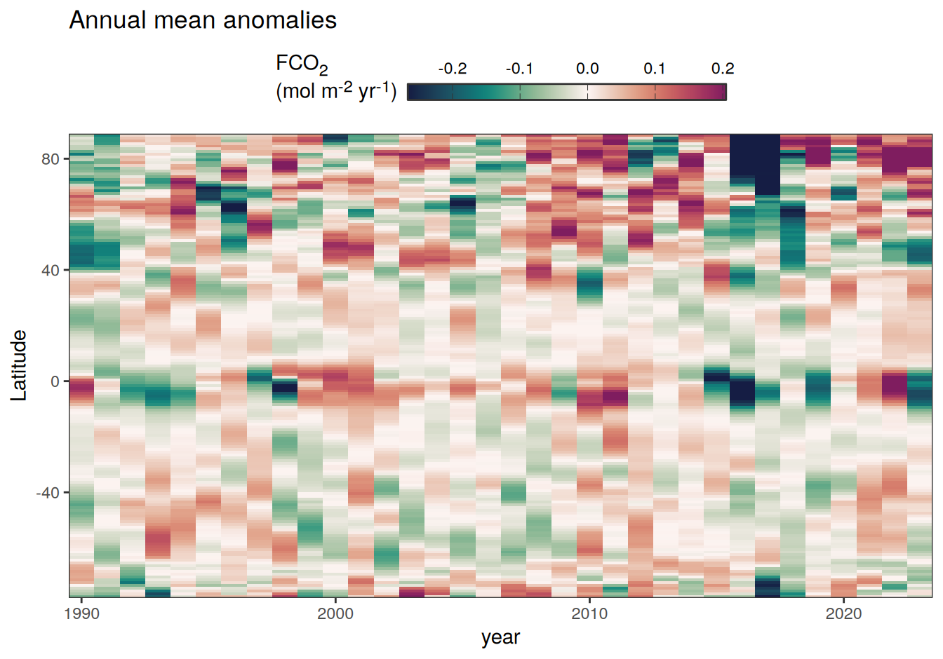
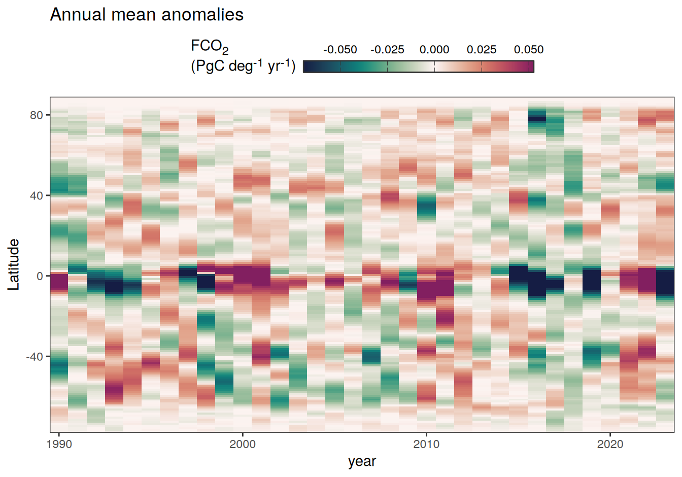
The following Hovmoeller plots show the value of each variable as provided through the pCO2 product. Hovmoeller plots are first presented as annual means, and than as monthly means.

Annual means

pco2_product_hovmoeller_annual <-
  pco2_product %>%
  mutate(fgco2_int = fgco2) %>% 
  select(-c(lon, time, month, biome)) %>%
  group_by(year, lat) %>%
  summarise(across(-c(fgco2_int, area),
                   ~ weighted.mean(., area, na.rm = TRUE)),
            across(fgco2_int,
                   ~ sum(. * area, na.rm = TRUE) * 12.01 * 1e-15)) %>%
  ungroup() %>%
  rename(fgco2_hov = fgco2_int) %>% 
  filter(fgco2_hov != 0)

pco2_product_hovmoeller_annual <-
  pco2_product_hovmoeller_annual %>%
  pivot_longer(-c(year, lat)) %>% 
  drop_na()

# pco2_product_hovmoeller_annual %>%
#   filter(!(name %in% name_divergent)) %>% 
#   group_split(name) %>%
#   # tail(5) %>%
#   map(
#     ~ ggplot(data = .x,
#              aes(year, lat, fill = value)) +
#       geom_raster() +
#       scale_fill_viridis_c(name = labels_breaks(.x %>% distinct(name))) +
#       theme(legend.title = element_markdown()) +
#       coord_cartesian(expand = 0) +
#       labs(title = "Annual means",
#            y = "Latitude") +
#       theme(axis.title.x = element_blank())
#   )
# 
# pco2_product_hovmoeller_annual %>%
#   filter(name %in% name_divergent) %>% 
#   group_split(name) %>%
#   # head(1) %>%
#   map(
#     ~ ggplot(data = .x,
#              aes(year, lat, fill = value)) +
#       geom_raster() +
#       scale_fill_gradientn(
#         colours = cmocean("curl")(100),
#         rescaler = ~ scales::rescale_mid(.x, mid = 0),
#         name = labels_breaks(.x %>% distinct(name)),
#         limits = c(quantile(.x$value, .01), quantile(.x$value, .99)),
#         oob = squish
#       ) +
#       theme(legend.title = element_markdown()) +
#       coord_cartesian(expand = 0) +
#       labs(title = "Annual means",
#            y = "Latitude") +
#       theme(axis.title.x = element_blank())
#   )

Monthly means

pco2_product_hovmoeller_monthly <-
  pco2_product %>%
  mutate(fgco2_int = fgco2) %>% 
  select(-c(lon, time, biome)) %>%
  group_by(year, month, lat) %>%
  summarise(across(-c(fgco2_int, area),
                   ~ weighted.mean(., area, na.rm = TRUE)),
            across(fgco2_int,
                   ~ sum(. * area, na.rm = TRUE) * 12.01 * 1e-15)) %>%
  ungroup() %>%
  rename(fgco2_hov = fgco2_int) %>% 
  filter(fgco2_hov != 0)


pco2_product_hovmoeller_monthly <-
  pco2_product_hovmoeller_monthly %>%
  pivot_longer(-c(year, month, lat)) %>% 
  drop_na()

pco2_product_hovmoeller_monthly <-
  pco2_product_hovmoeller_monthly %>% 
  mutate(decimal = year + (month-1) / 12)

# pco2_product_hovmoeller_monthly %>%
#   filter(!(name %in% name_divergent)) %>%
#   group_split(name) %>%
#   # head(1) %>%
#   map(
#     ~ ggplot(data = .x,
#              aes(decimal, lat, fill = value)) +
#       geom_raster() +
#       scale_fill_viridis_c(name = labels_breaks(.x %>% distinct(name))) +
#       theme(legend.title = element_markdown()) +
#       labs(title = "Monthly means",
#            y = "Latitude") +
#       coord_cartesian(expand = 0) +
#       theme(axis.title.x = element_blank())
#   )
# 
# pco2_product_hovmoeller_monthly %>%
#   filter(name %in% name_divergent) %>%
#   group_split(name) %>%
#   # head(1) %>%
#   map(
#     ~ ggplot(data = .x,
#              aes(decimal, lat, fill = value)) +
#       geom_raster() +
#       scale_fill_gradientn(
#         colours = cmocean("curl")(100),
#         rescaler = ~ scales::rescale_mid(.x, mid = 0),
#         name = labels_breaks(.x %>% distinct(name)),
#         limits = c(quantile(.x$value, .01), quantile(.x$value, .99)),
#         oob = squish
#       )+
#       theme(legend.title = element_markdown()) +
#       labs(title = "Monthly means",
#            y = "Latitude") +
#       coord_cartesian(expand = 0) +
#       theme(axis.title.x = element_blank())
#   )

rm(pco2_product)

gc()

pCO2_product_analysis_2023 <-
  knitr::knit_expand(
    file = here::here("analysis/child/pCO2_product_analysis.Rmd"),
    product_name = "NIES-ML3_GCB",
    year_anom = 2023
  )

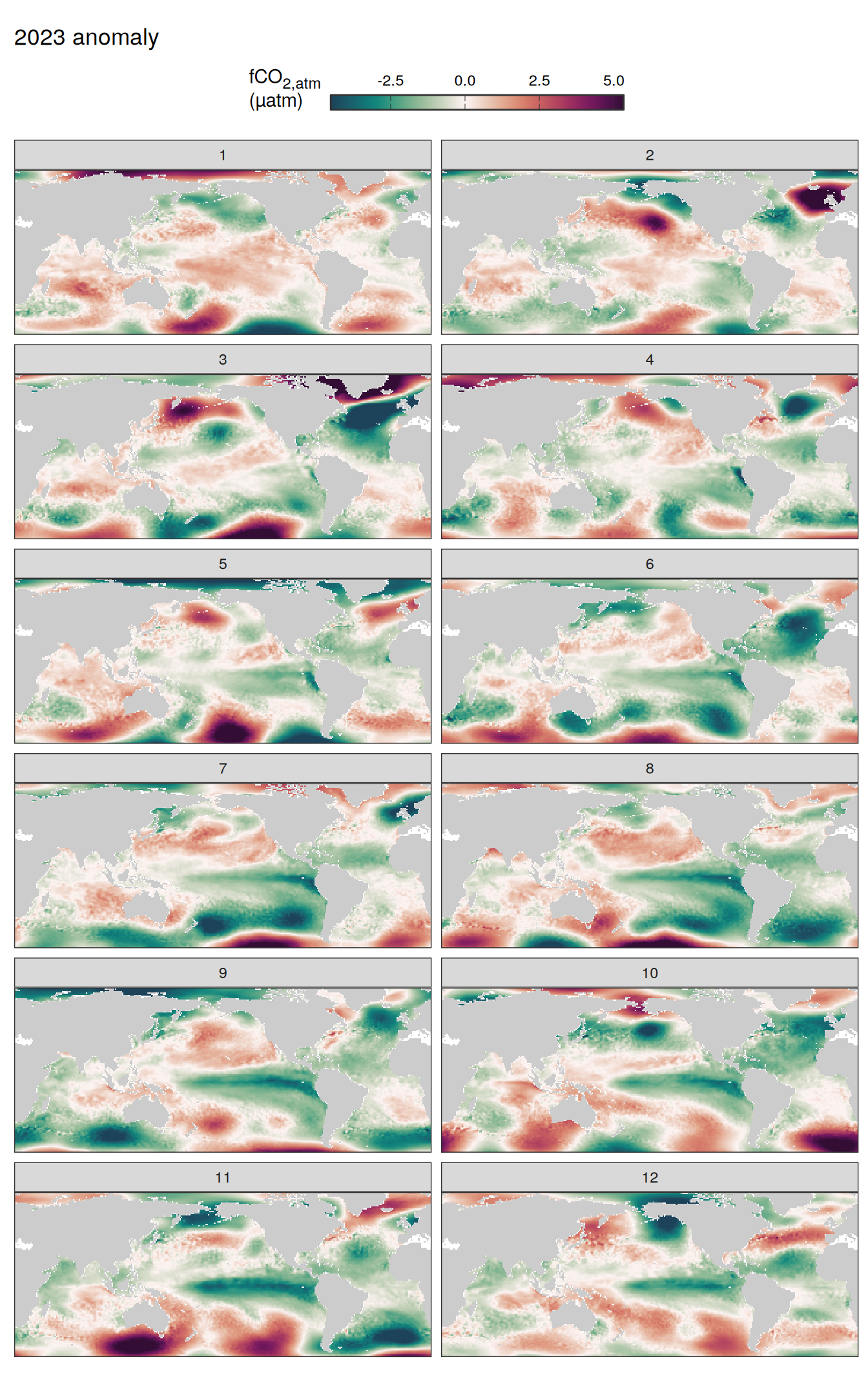
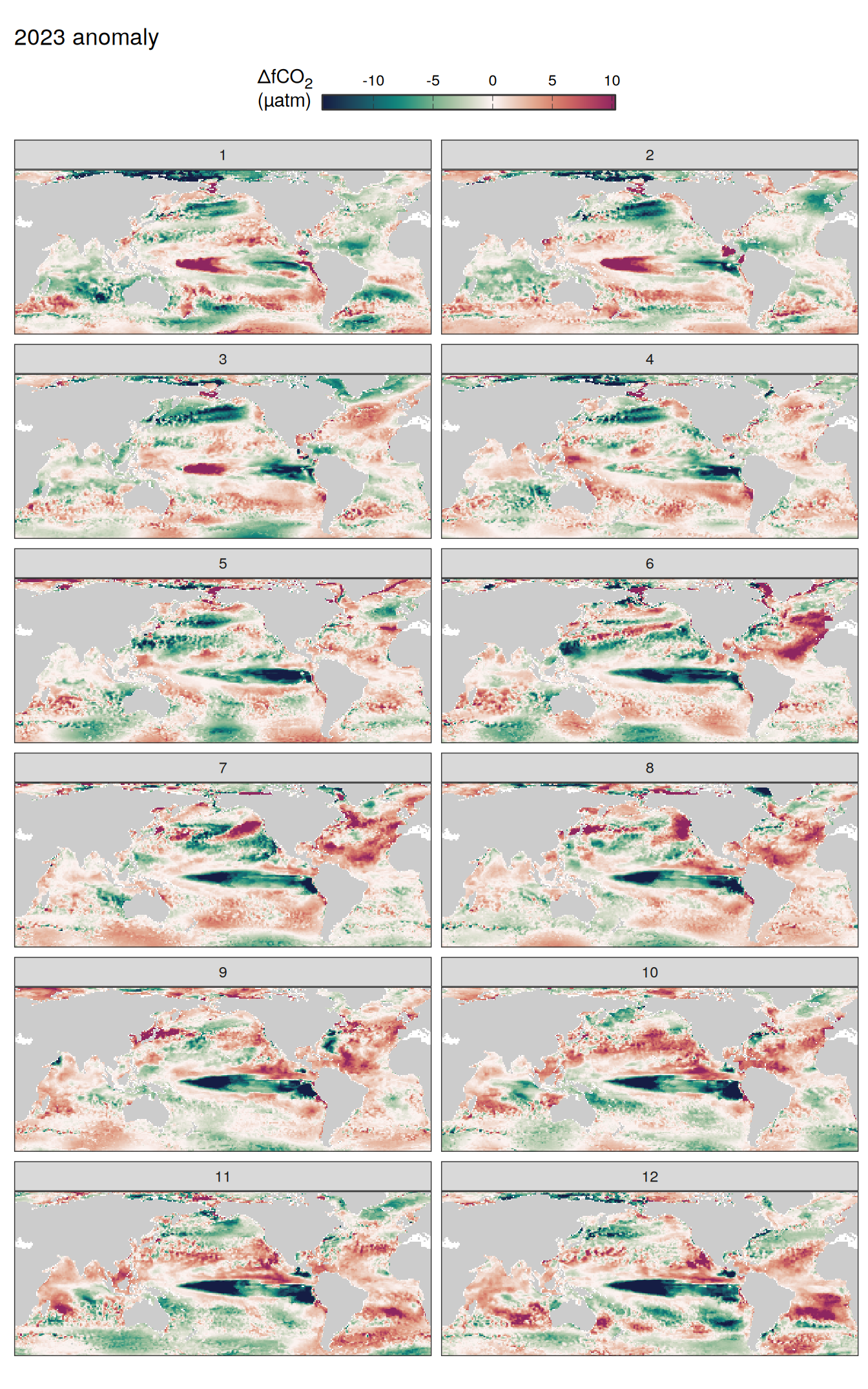
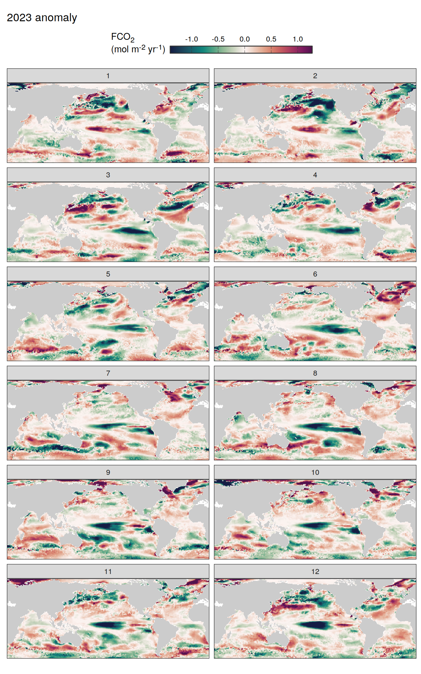
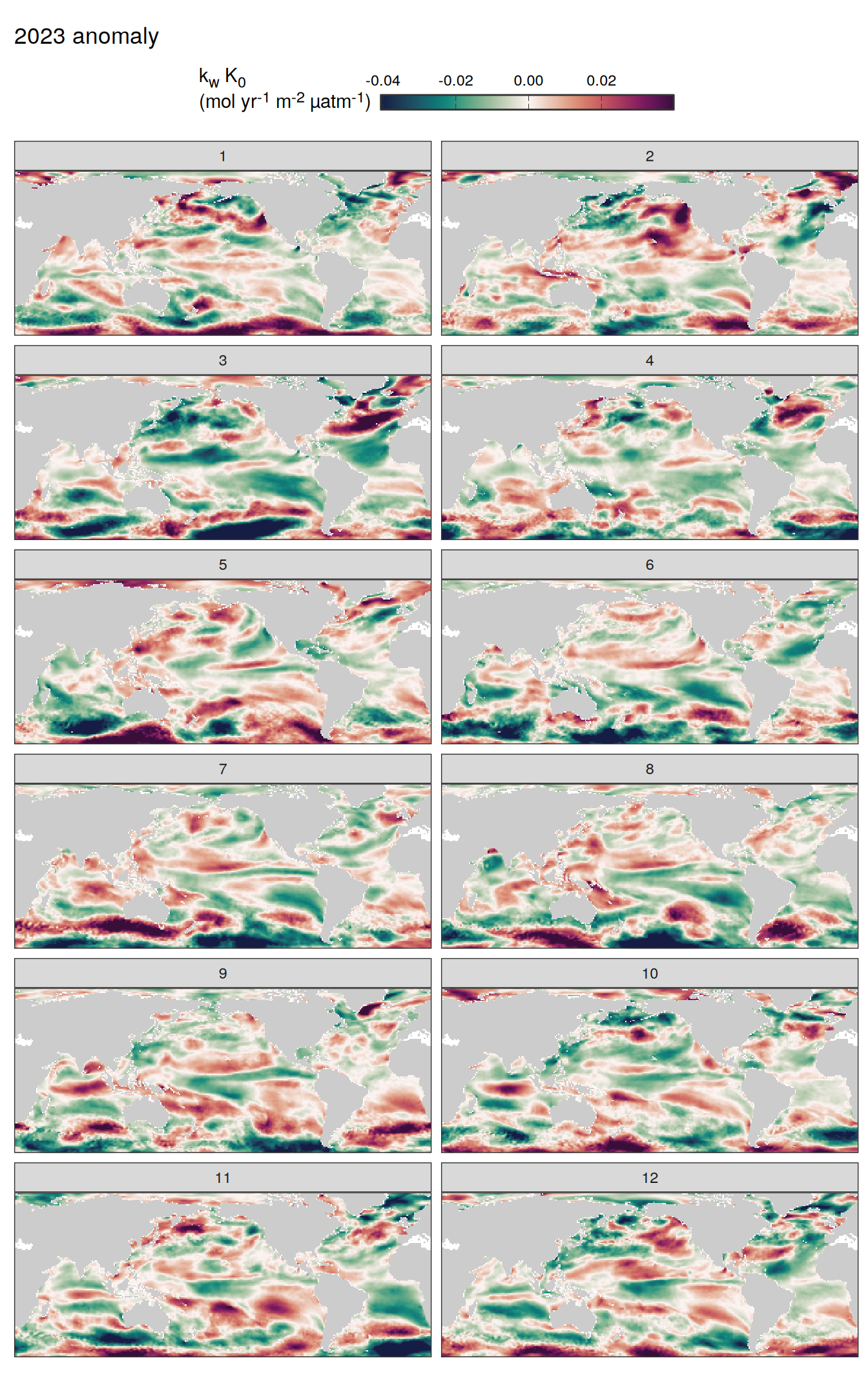
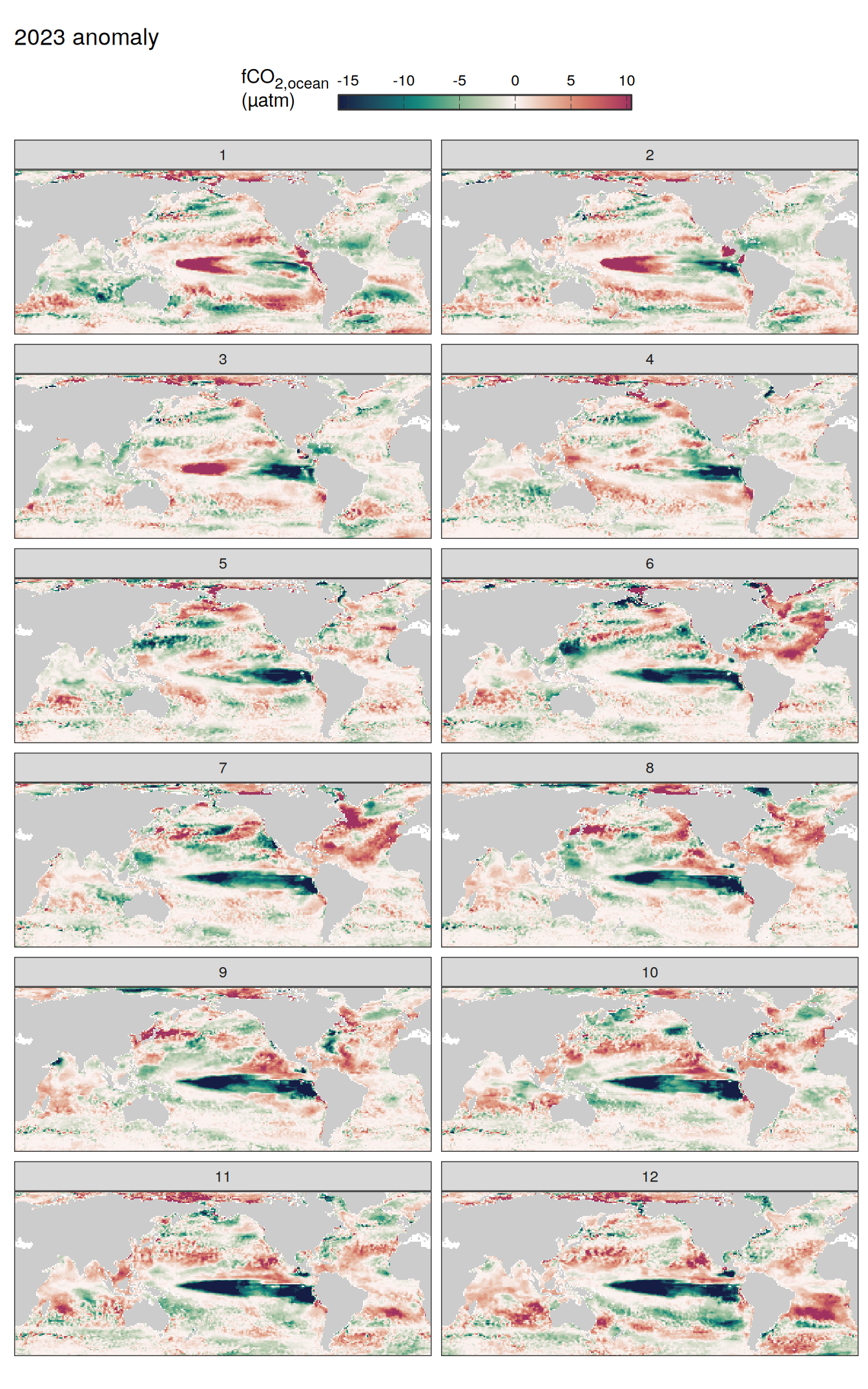
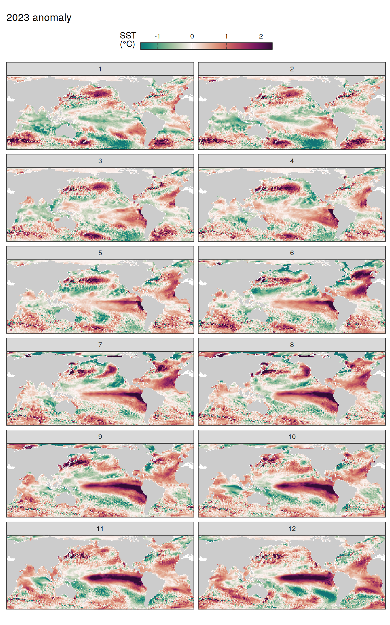
2023 anomalies

Functions

Anomaly detection

For the detection of anomalies at any point in time and space, we fit regression models and compare the fitted to the actual value.

We use linear regression models for all parameters, except for , which are approximated with quadratic fits.

The regression models are fitted to all data since , except 2023.

anomaly_determination <- function(df,...) {
  
  group_by <- quos(...)
  # group_by <- quos(lon, lat)
  # group_by <- quos(biome)
  # df <- pco2_product_map_annual
  # Linear regression models

  df_lm <-
    df %>%
    filter(year != 2023,
           !(name %in% name_quadratic_fit)) %>%
    drop_na() %>%
    nest(data = -c(name, !!!group_by)) %>%
    mutate(fit = map(data, ~ flm(
      formula = value ~ year, data = .x
    )))
  
  df_lm <-
    left_join(
      df_lm %>%
        unnest_wider(fit) %>%
        select(name, !!!group_by,
               intercept = `(Intercept)`,  slope = year) %>%
        mutate(intercept = as.vector(intercept),
               slope = as.vector(slope)),
      df
    ) %>%
    mutate(fit = intercept + year * slope) %>%
    select(name, !!!group_by, year, fit, value) %>%
    mutate(resid = value - fit)

  # df_lm <-
  #   df %>%
  #   filter(year != 2023,
  #          !(name %in% name_quadratic_fit)) %>%
  #   drop_na() %>% 
  #   nest(data = -c(name, !!!group_by)) %>%
  #   mutate(
  #     fit = map(data, ~ lm(value ~ year, data = .x)),
  #     tidied = map(fit, tidy),
  #     augmented = map(fit, augment)
  #   )
  # 
  # 
  # df_lm_year_anom <-
  #   full_join(
  #     df_lm %>%
  #       unnest(tidied) %>%
  #       select(name, !!!group_by, term, estimate) %>%
  #       pivot_wider(names_from = term,
  #                   values_from = estimate) %>%
  #       mutate(fit = `(Intercept)` + year * 2023) %>%
  #       select(name, !!!group_by, fit) %>%
  #       mutate(year = 2023),
  #     df %>%
  #       filter(year == 2023,
  #              !(name %in% name_quadratic_fit))
  #   ) %>%
  #   mutate(resid = value - fit)
  # 
  # 
  # df_lm <-
  #   bind_rows(
  #     df_lm %>%
  #       unnest(augmented) %>%
  #       select(name, !!!group_by, year, value, fit = .fitted, resid = .resid),
  #     df_lm_year_anom
  #   )
  # 
  # rm(df_lm_year_anom)
  
  # Quadratic regression models
  
  if(any(df %>% distinct(name) %>% pull() %in% name_quadratic_fit)){
  
  df_quadratic <-
    df %>%
    filter(year != 2023,
           name %in% name_quadratic_fit) %>%
    drop_na() %>% 
    mutate(year = year - 2000) %>% 
    nest(data = -c(name, !!!group_by)) %>%
    mutate(
      fit = map(data, ~ flm(
        # formula = value ~ year + I(year ^ 2), data = .x))
        # formula = value ~ year + I(year ^ 2) + I(year ^ 3), data = .x))
        formula = value ~ poly(year, 2, raw = TRUE), data = .x))
    )
  
  df_quadratic <-
    left_join(
      df_quadratic %>%
        unnest_wider(fit) %>%
        select(name, !!!group_by,
               intercept = `(Intercept)`,
               slope = `1`, 
               slope_squared = `2`
               # slope_cube = `3`
               ) %>%
        mutate(intercept = as.vector(intercept),
               slope = as.vector(slope),
               slope_squared = as.vector(slope_squared)
               # slope_cube = as.vector(slope_cube)
               ),
      df %>% 
        mutate(year = year - 2000)
    ) %>%
    mutate(fit = intercept + year * slope + year^2 * slope_squared) %>%
    select(name, !!!group_by, year, fit, value) %>%
    mutate(resid = value - fit,
           year = year + 2000)
  
  
  # df_quadratic <-
  #   df %>%
  #   filter(year != 2023,
  #          name %in% name_quadratic_fit) %>%
  #   nest(data = -c(name, !!!group_by)) %>%
  #   mutate(
  #     fit = map(data, ~ lm(value ~ year + I(year ^ 2), data = .x)),
  #     tidied = map(fit, tidy),
  #     augmented = map(fit, augment)
  #   )
  # 
  # df_quadratic_year_anom <-
  #   full_join(
  #     df_quadratic %>%
  #       unnest(tidied) %>%
  #       select(name, !!!group_by, term, estimate) %>%
  #       pivot_wider(names_from = term,
  #                   values_from = estimate) %>%
  #       mutate(fit = `(Intercept)` + year * 2023 + `I(year^2)` * 2023 ^ 2) %>%
  #       select(name, !!!group_by, fit) %>%
  #       mutate(year = 2023),
  #     df %>%
  #       filter(year == 2023,
  #              name %in% name_quadratic_fit)
  #   ) %>%
  #   mutate(resid = value - fit)
  # 
  # 
  # df_quadratic <-
  #   bind_rows(
  #     df_quadratic %>%
  #       unnest(augmented) %>%
  #       select(name, !!!group_by, year, value, fit = .fitted, resid = .resid),
  #     df_quadratic_year_anom
  #   )
  # 
  # rm(df_quadratic_year_anom)
  
  # Join linear and quadratic regression results
  
  df_anomaly <-
    bind_rows(df_lm,
              df_quadratic)
  
  rm(df_lm,
     df_quadratic)
  
  } else{
    
    df_anomaly <- df_lm
    
    rm(df_lm)
  }
  
  df_anomaly <-
    df_anomaly %>%
    arrange(year)
  
  
  return(df_anomaly)
  
}

Seasonality plots

warm_color <- "#B84A60FF"
cold_color <- "#16877CFF"

p_season <- function(df, 
                     dim_row = "name", 
                     dim_col = "biome", 
                     title = NULL, 
                     var = "resid",
                     scales = "free_y") {
  
  p <- ggplot(data = df,
              aes(month, !!ensym(var)))
  
  if(var == "resid"){
      p <- p +
        geom_hline(yintercept = 0, linewidth =0.5)
    
  }
  
  
  
  p <- p +
      geom_path(data = . %>% filter(year != 2023),
                aes(group = as.factor(year),
                    col = as.factor(paste(min(year), max(year), sep = "-"))), 
                alpha = 0.5)+
      geom_path(data = . %>% 
                  filter(year != 2023) %>% 
                  group_by_at(vars(month, dim_col, dim_row)) %>% 
                  summarise(!!ensym(var) := mean(!!ensym(var))),
                aes(col = "Climatological\nmean"), 
                linewidth = 1) +
    scale_color_manual(values = c("grey", "black"),
                       guide = guide_legend(order = 2,
                                            reverse = TRUE)) +
    new_scale_color()+
    geom_path(data = . %>% filter(year == 2023),
                aes(col = as.factor(year)),
                linewidth = 1) +
      scale_color_manual(
        values = warm_color,
        guide = guide_legend(order = 1)
      ) +
      scale_x_continuous(breaks = seq(1, 12, 3), expand = c(0, 0)) +
      labs(title = title,
           x = "Month")
  
    if(df %>% filter(name == "fgco2") %>% nrow() > 0 & "value" %in% names(df)){
    
    df_sink <- df %>% 
      filter(year == 2023,
             name == "fgco2")
    
      p <- p +
          geom_point(data = df_sink %>% filter(value < 0),
             aes(shape = "Sink"), fill = "white") +
          geom_point(data = df_sink %>% filter(value >= 0),
             aes(shape = "Source"), fill = "white") +
        scale_shape_manual(values = c(25,24))
    
  }
  
  
  if (!(is.null(dim_col))) {
    p <- p +
      facet_grid(
        as.formula(paste(dim_row, "~", dim_col)),
        scales = scales,
        labeller = labeller(name = x_axis_labels),
        switch = "y"
      )
    
    
  } else {
    p <- p +
      facet_grid(
        as.formula(paste(dim_row, "~ .")),
        scales = "free_y",
        labeller = labeller(name = x_axis_labels),
        switch = "y"
      )
  }
  
  p <- p +
    theme(
      strip.text.y.left = element_markdown(),
      strip.placement = "outside",
      strip.background.y = element_blank(),
      axis.title.y = element_blank(),
      legend.title = element_blank()
    )
  
  p
  
}

fCO2 decomposition

fco2_decomposition <- function(df, ...) {
  
  group_by <- quos(...)
  # group_by <- quos(lon, lat, month)
  # group_by <- quos(biome, year, month)
  
  pco2_product_biome_monthly_fCO2_decomposition <-
    df %>%
    filter(name %in% c("temperature", "sfco2"))
  
  pco2_product_biome_monthly_fCO2_decomposition <-
    inner_join(
      pco2_product_biome_monthly_fCO2_decomposition %>%
        filter(name == "temperature") %>%
        select(-c(value, fit)) %>%
        pivot_wider(values_from = resid),
      pco2_product_biome_monthly_fCO2_decomposition %>%
        filter(name == "sfco2") %>%
        select(-c(value, resid)) %>%
        pivot_wider(values_from = fit)
    )
  
  pco2_product_biome_monthly_fCO2_decomposition <-
    pco2_product_biome_monthly_fCO2_decomposition %>%
    mutate(sfco2_therm = (sfco2 * exp(0.0423 * temperature)) - sfco2)
  
  
  pco2_product_biome_monthly_fCO2_decomposition <-
    inner_join(
      pco2_product_biome_monthly_fCO2_decomposition,
      df %>%
        filter(name %in% c("sfco2")) %>%
        select(-c(value, fit, name)) %>%
        rename(sfco2_total = resid)
    )
  
  
  pco2_product_biome_monthly_fCO2_decomposition <-
    pco2_product_biome_monthly_fCO2_decomposition %>%
    mutate(sfco2_nontherm = sfco2_total - sfco2_therm)
  
  pco2_product_biome_monthly_fCO2_decomposition <-
    pco2_product_biome_monthly_fCO2_decomposition %>%
    select(-c(temperature, sfco2)) %>%
    pivot_longer(starts_with("sfco2"),
                 values_to = "resid")
  
}

fco2_decomposition <- function(df, ...) {
  
  group_by <- quos(...)
  # group_by <- quos(lon, lat, month)
  # group_by <- quos(biome, year, month)
  
  pco2_product_biome_monthly_fCO2_decomposition <-
    df %>%
    filter(name %in% c("temperature", "sfco2"))
  
  pco2_product_biome_monthly_fCO2_decomposition <-
    inner_join(
      pco2_product_biome_monthly_fCO2_decomposition %>%
        filter(name == "temperature") %>%
        select(-c(value, fit)) %>%
        pivot_wider(values_from = resid),
      pco2_product_biome_monthly_fCO2_decomposition %>%
        filter(name == "sfco2") %>%
        select(-c(value, resid)) %>%
        pivot_wider(values_from = fit)
    )
  
  pco2_product_biome_monthly_fCO2_decomposition <-
    pco2_product_biome_monthly_fCO2_decomposition %>%
    mutate(
      sfco2_therm = (sfco2 * exp(0.0423 * temperature)) - sfco2,
      sfco2_nontherm = (sfco2 * exp(-0.0423 * temperature)) - sfco2)
  
  
  pco2_product_biome_monthly_fCO2_decomposition <-
    inner_join(
      pco2_product_biome_monthly_fCO2_decomposition,
      df %>%
        filter(name %in% c("sfco2")) %>%
        select(-c(value, fit, name)) %>%
        rename(sfco2_total = resid)
    )
  
  
  # pco2_product_biome_monthly_fCO2_decomposition <-
  #   pco2_product_biome_monthly_fCO2_decomposition %>%
  #   mutate(sfco2_nontherm = sfco2_total - sfco2_therm)
  
  pco2_product_biome_monthly_fCO2_decomposition <-
    pco2_product_biome_monthly_fCO2_decomposition %>%
    select(-c(temperature, sfco2)) %>%
    pivot_longer(starts_with("sfco2"),
                 values_to = "resid")
  
}

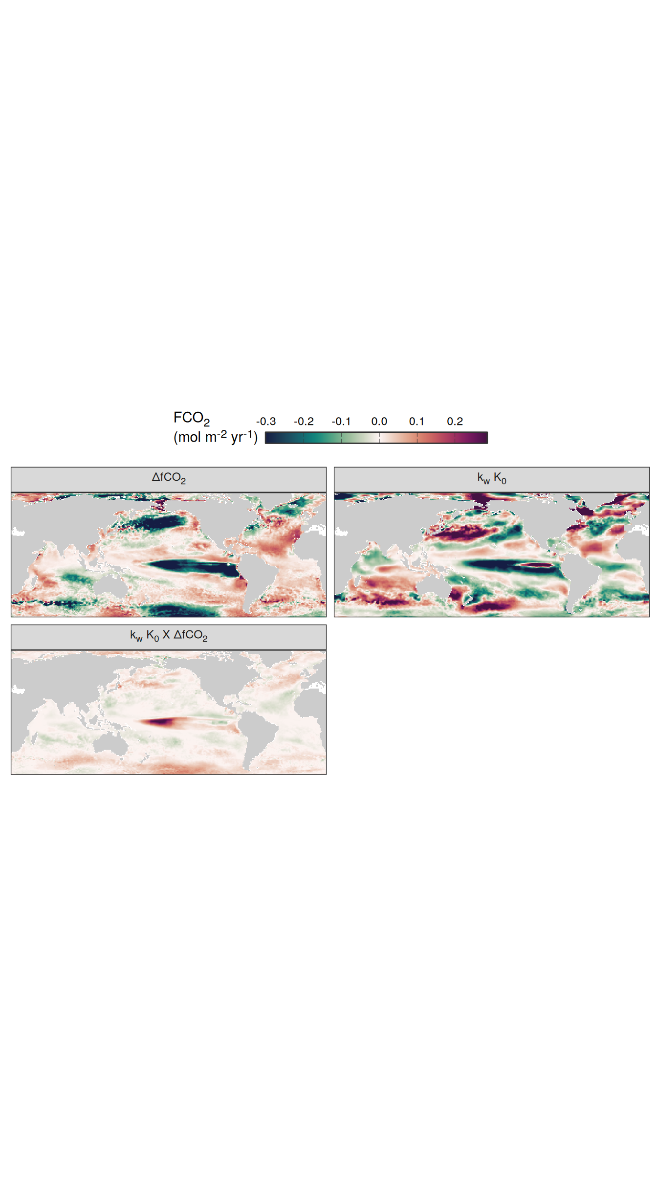
Flux attribution

flux_attribution <- function(df, ...) {
  
  group_by <- quos(...)
  # group_by <- quos(lon, lat, month)
  
  pco2_product_flux_attribution <-
    df %>%
    filter(name %in% c("dfco2", "kw_sol", "fgco2"))
  
  
  pco2_product_flux_attribution <-
    inner_join(
      pco2_product_flux_attribution %>%
        select(-c(value, fit)) %>%
        pivot_wider(values_from = resid,
                    names_prefix = "resid_"),
      pco2_product_flux_attribution %>%
        select(-c(value, resid)) %>%
        filter(name != "fgco2") %>%
        pivot_wider(values_from = fit)
    )
  
    pco2_product_flux_attribution <-
    pco2_product_flux_attribution %>%
    mutate(
      resid_fgco2_dfco2 = resid_dfco2 * kw_sol,
      resid_fgco2_kw_sol = resid_kw_sol * dfco2,
      resid_fgco2_dfco2_kw_sol = resid_dfco2 * resid_kw_sol
      # resid_fgco2_sum = resid_fgco2_dfco2 + resid_fgco2_kw_sol + resid_fgco2_dfco2_kw_sol
    )
  
  # pco2_product_flux_attribution <-
  #   pco2_product_flux_attribution %>%
  #   mutate(resid_fgco2_offset = resid_fgco2 - resid_fgco2_sum)
  
  pco2_product_flux_attribution <-
    pco2_product_flux_attribution %>%
    select(!!!group_by, starts_with("resid_fgco2")) %>%
    pivot_longer(starts_with("resid_"),
                 values_to = "resid")
  
  
  pco2_product_flux_attribution <-
    pco2_product_flux_attribution %>%
    filter(str_detect(name, "dfco2|kw_sol")) %>% 
    mutate(name = factor(
      name,
      levels = c(
        "resid_fgco2",
        "resid_fgco2_dfco2",
        "resid_fgco2_kw_sol",
        "resid_fgco2_dfco2_kw_sol",
        "resid_fgco2_sum",
        "resid_fgco2_offset"
      )
    ))
  
}

Maps

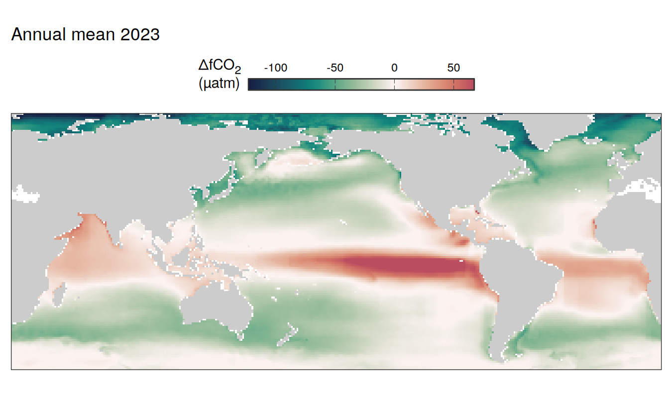
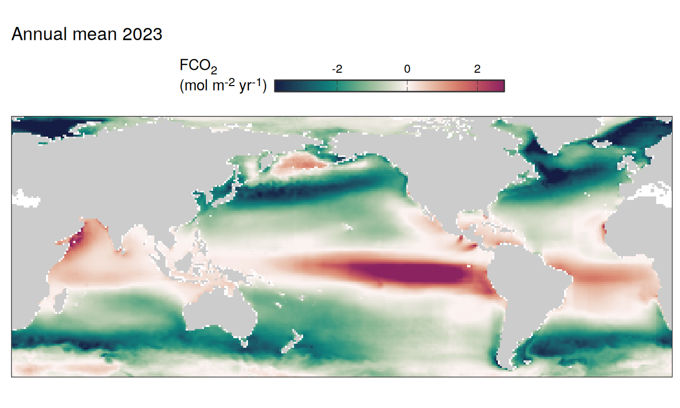
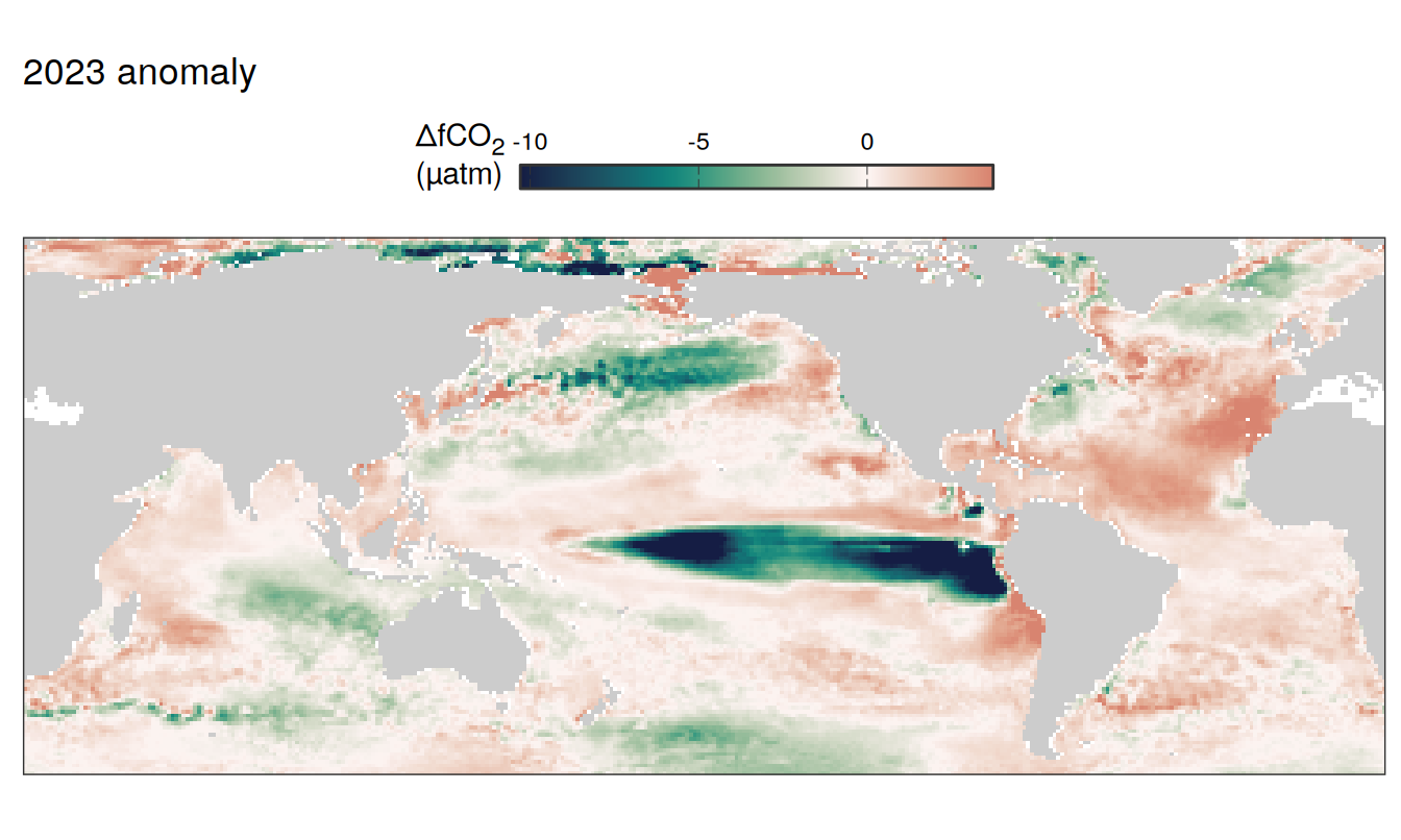
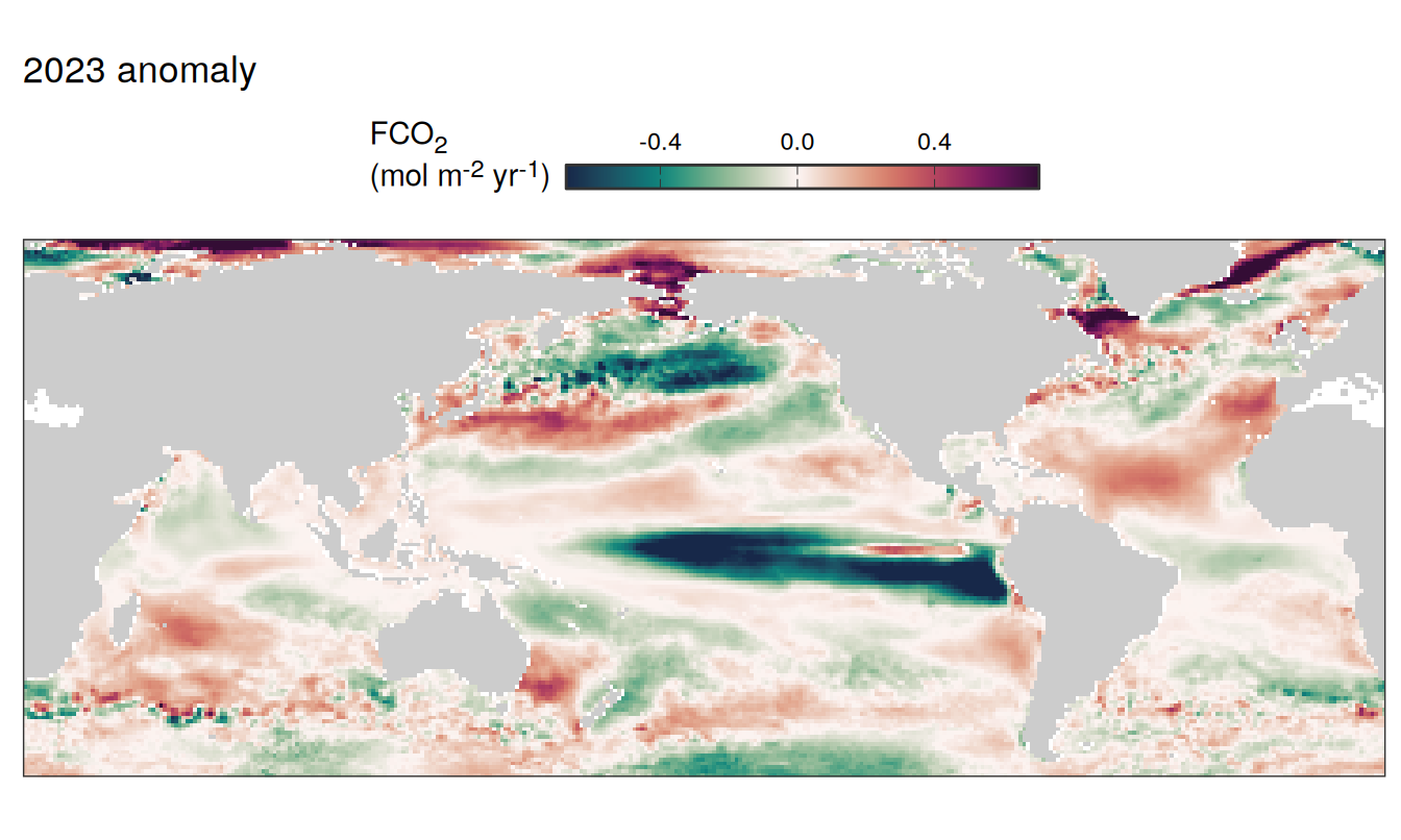
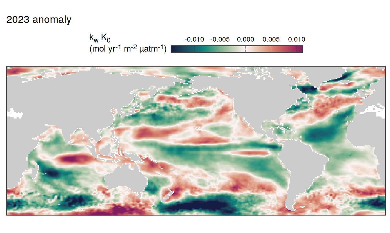
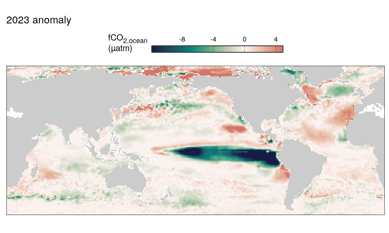
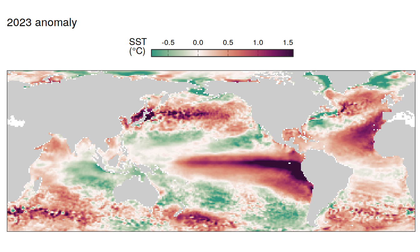
The following maps show the absolute state of each variable in 2023 as provided through the pCO2 product, the change in that variable from 1990 to 2023, as well es the anomalies in 2023. Changes and anomalies are determined based on the predicted value of a linear regression model fit to the data from 1990 to 2022.

Maps are first presented as annual means, and than as monthly means. Note that the 2023 predictions for the monthly maps are done individually for each month, such the mean seasonal anomaly from the annual mean is removed.

Note: The increase the computational speed, I regridded all maps to 5X5° grid.

Annual means

2023 absolute

pco2_product_map_annual_anomaly <-
  pco2_product_map_annual %>%
  drop_na() %>% 
  anomaly_determination(lon, lat)

pco2_product_map_annual_anomaly <-
  pco2_product_map_annual_anomaly %>%
  drop_na()

pco2_product_map_annual_anomaly %>%
  filter(year == 2023,
         !(name %in% name_divergent)) %>%
  group_split(name) %>%
  # head(1) %>%
  map(
    ~ map +
      geom_tile(data = .x,
                aes(lon, lat, fill = value)) +
      labs(title = paste("Annual mean", 2023)) +
      scale_fill_viridis_c(name = labels_breaks(.x %>% distinct(name))) +
      guides(
        fill = guide_colorbar(
          barheight = unit(0.3, "cm"),
          barwidth = unit(6, "cm"),
          ticks = TRUE,
          ticks.colour = "grey20",
          frame.colour = "grey20",
          label.position = "top",
          direction = "horizontal"
        )
      ) +
      theme(legend.title = element_markdown(),
            legend.position = "top")
  )

pco2_product_map_annual_anomaly %>%
  filter(year == 2023,
         name %in% name_divergent) %>%
  group_split(name) %>% 
  # head(1) %>%
  map( ~ map +
         geom_tile(data = .x,
                   aes(lon, lat, fill = value)) +
         labs(title = paste("Annual mean", 2023)) +
         scale_fill_gradientn(
           colours = cmocean("curl")(100),
           rescaler = ~ scales::rescale_mid(.x, mid = 0),
           name = labels_breaks(.x %>% distinct(name)),
           limits = c(quantile(.x$value, .01), quantile(.x$value, .99)),
           oob = squish
         ) +
      guides(
        fill = guide_colorbar(
          barheight = unit(0.3, "cm"),
          barwidth = unit(6, "cm"),
          ticks = TRUE,
          ticks.colour = "grey20",
          frame.colour = "grey20",
          label.position = "top",
          direction = "horizontal"
        )
      ) +
      theme(legend.title = element_markdown(),
            legend.position = "top")
  )

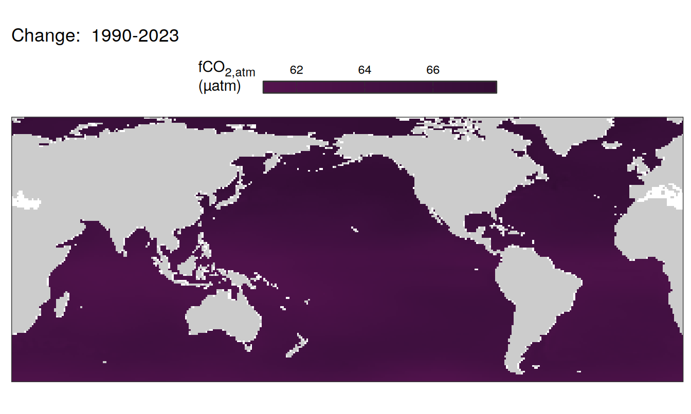
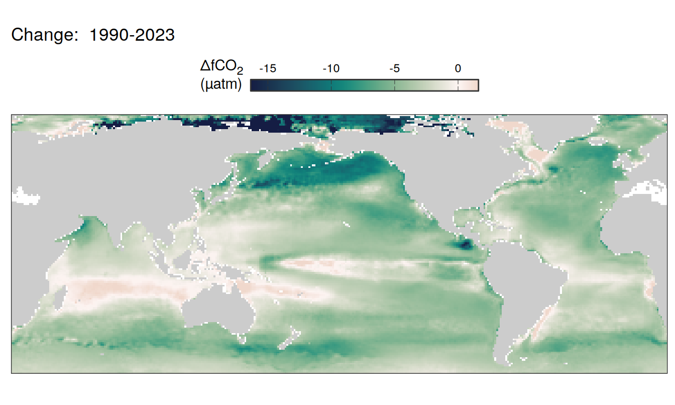
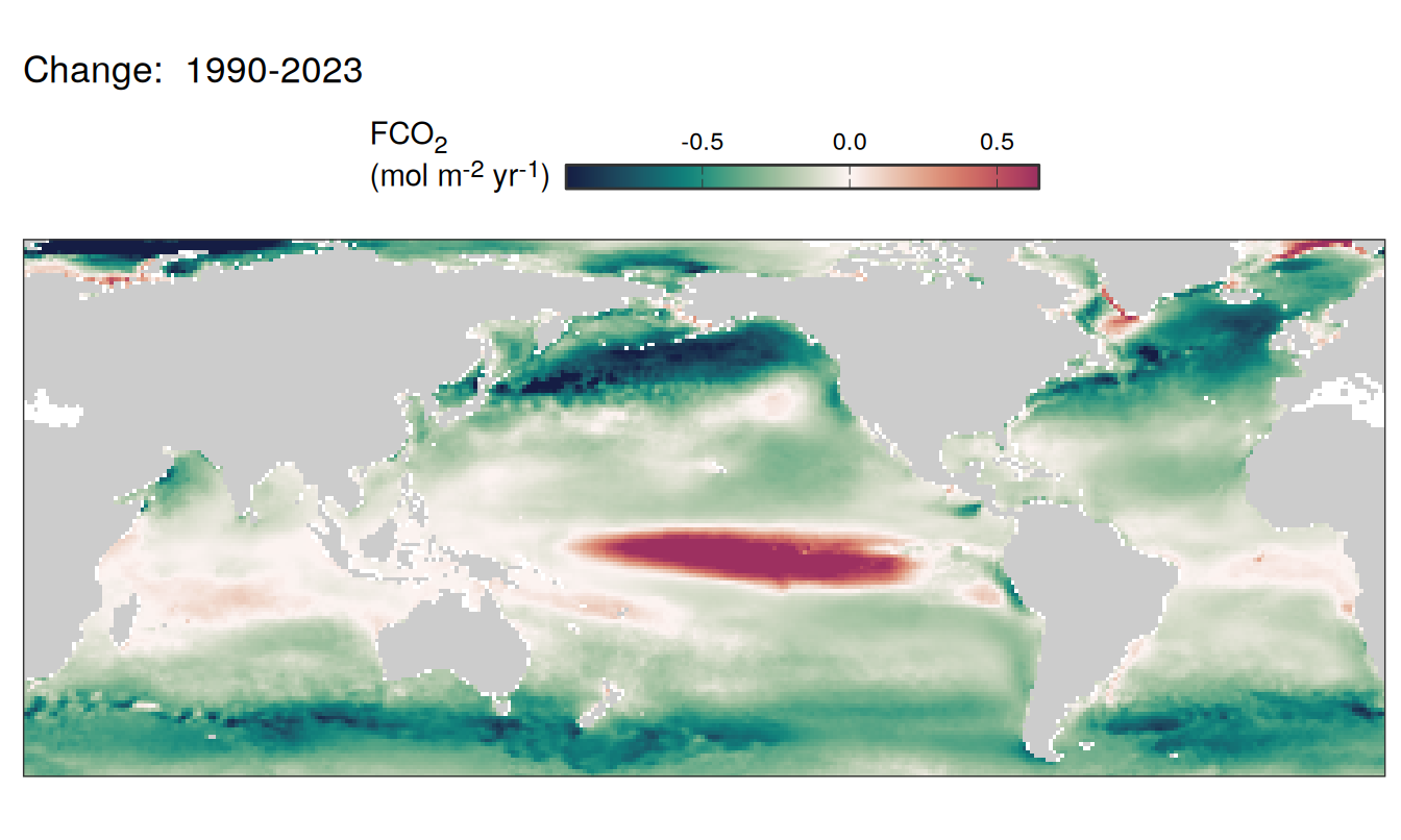
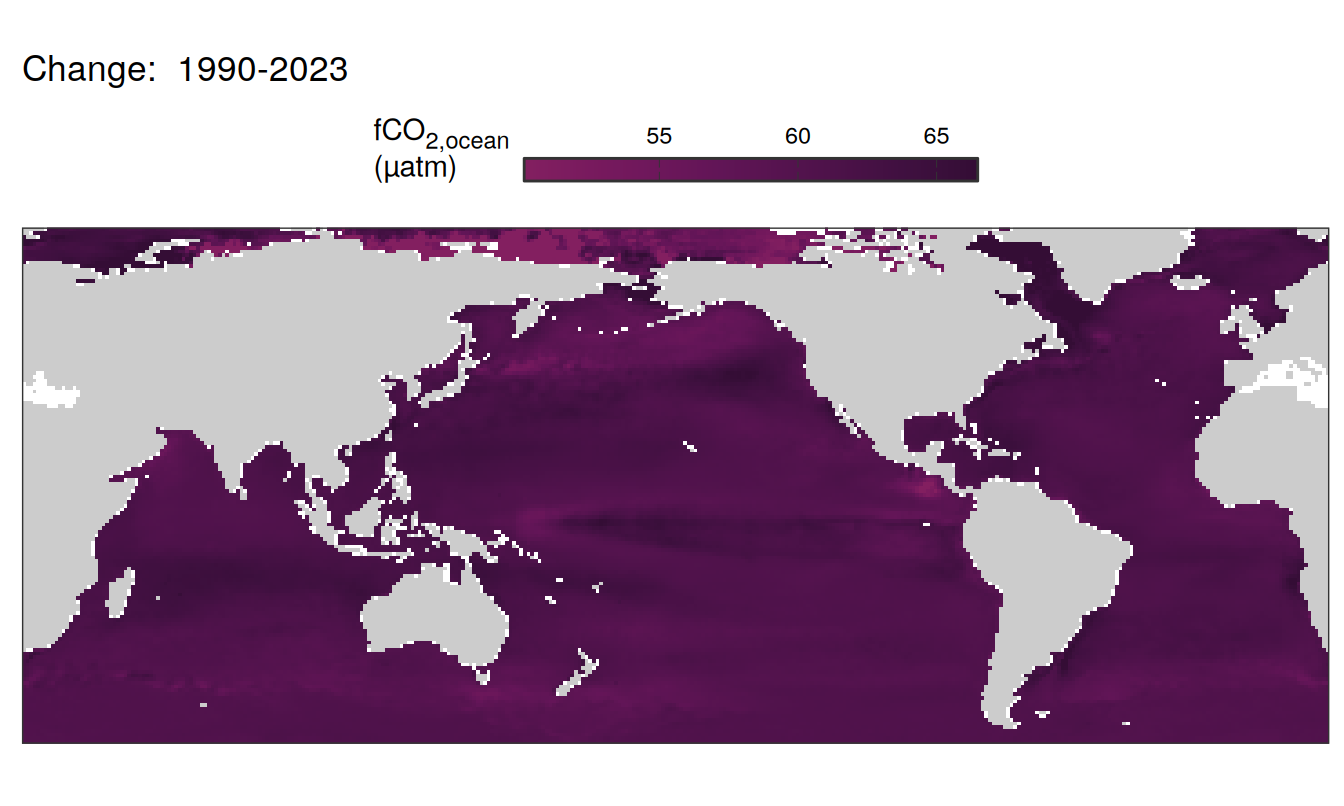
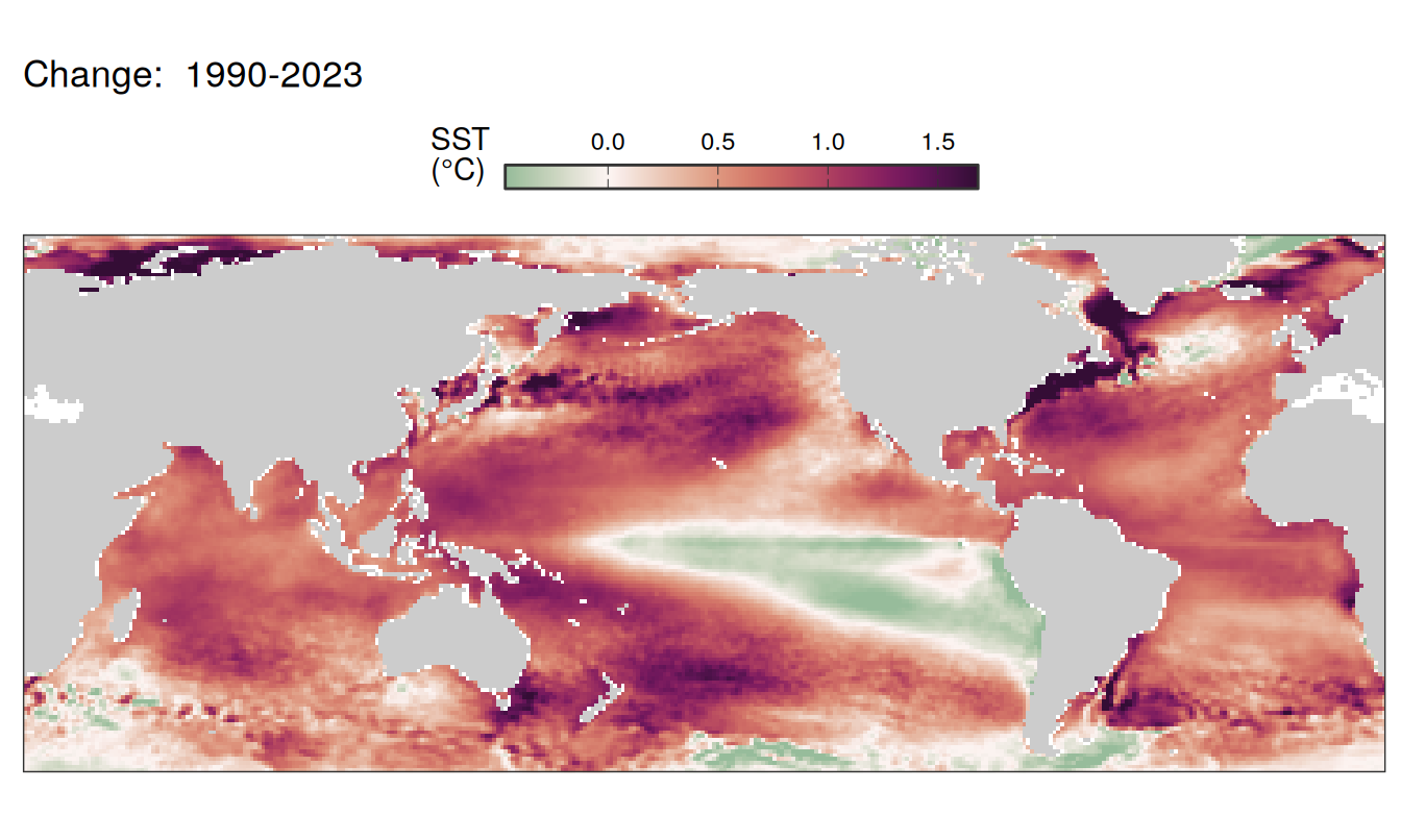
Trends

pco2_product_map_annual_anomaly %>%
  group_by(name) %>%
  filter(year %in% c(min(year), max(year), 2023)) %>%
  ungroup() %>%
  select(-c(value, resid)) %>%
  filter(year %in% c(min(year), max(year))) %>%
  arrange(year) %>% 
  group_by(lon, lat, name) %>%
  mutate(change = fit - lag(fit),
         period = paste(lag(year), year, sep = "-")) %>%
  ungroup() %>%
  filter(!is.na(change)) %>%
  group_split(name) %>% 
  # head(1) %>%
  map(
    ~ map +
      geom_tile(data = .x,
                aes(lon, lat, fill = change)) +
      labs(title =  paste("Change: ",.x$period)) +
      scale_fill_gradientn(
        colours = cmocean("curl")(100),
        rescaler = ~ scales::rescale_mid(.x, mid = 0),
        name = labels_breaks(.x %>% distinct(name)),
        limits = c(quantile(.x$change, .01), quantile(.x$change, .99)),
        oob = squish
      ) +
      guides(
        fill = guide_colorbar(
          barheight = unit(0.3, "cm"),
          barwidth = unit(6, "cm"),
          ticks = TRUE,
          ticks.colour = "grey20",
          frame.colour = "grey20",
          label.position = "top",
          direction = "horizontal"
        )
      ) +
      theme(legend.title = element_markdown(),
            legend.position = "top")
  )

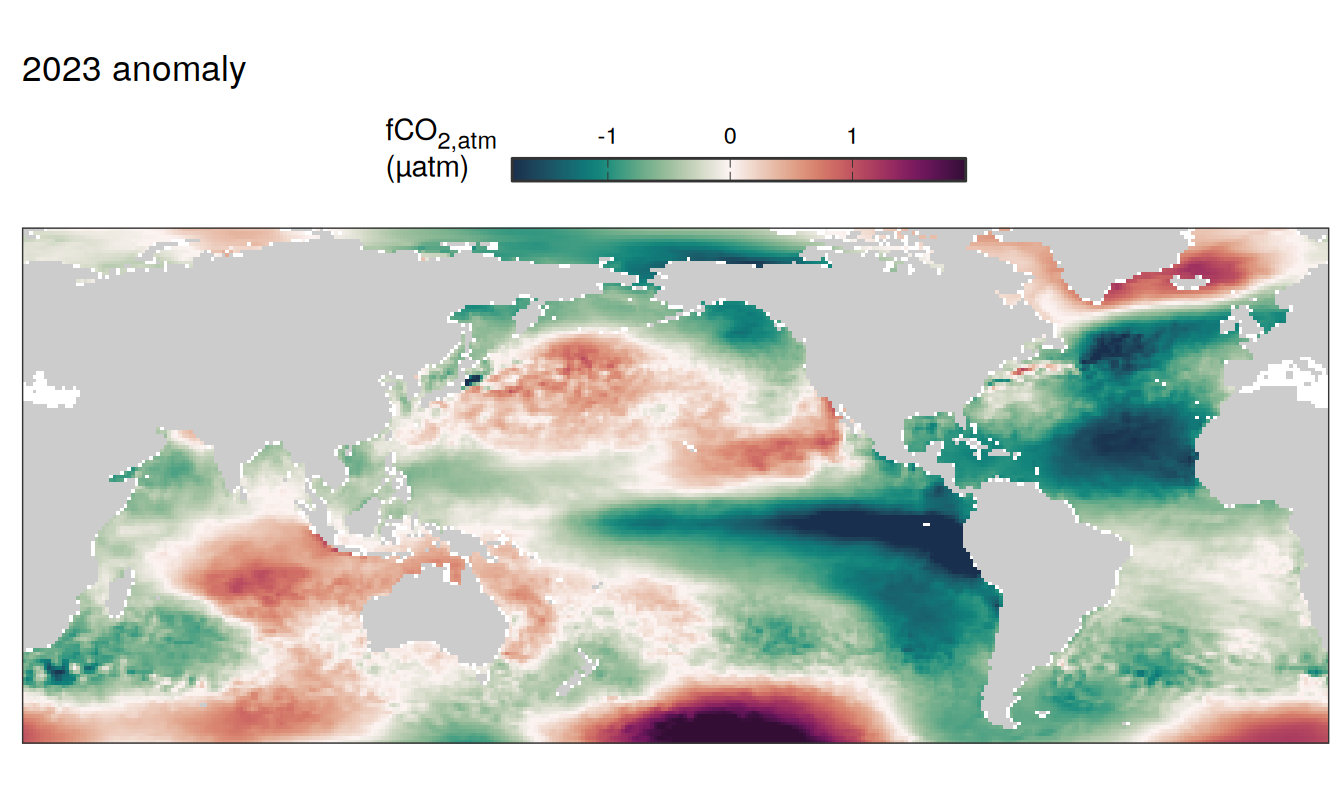
2023 anomaly

pco2_product_map_annual_anomaly %>%
  filter(year == 2023) %>%
  group_split(name) %>% 
  # head(1) %>%
  map( ~ map +
         geom_tile(data = .x,
                   aes(lon, lat, fill = resid)) +
         labs(title =  paste(2023,"anomaly")) +
         scale_fill_gradientn(
           colours = cmocean("curl")(100),
           rescaler = ~ scales::rescale_mid(.x, mid = 0),
           name = labels_breaks(.x %>% distinct(name)),
           limits = c(quantile(.x$resid, .01), quantile(.x$resid, .99)),
           oob = squish
         )+
      guides(
        fill = guide_colorbar(
          barheight = unit(0.3, "cm"),
          barwidth = unit(6, "cm"),
          ticks = TRUE,
          ticks.colour = "grey20",
          frame.colour = "grey20",
          label.position = "top",
          direction = "horizontal"
        )
      ) +
      theme(legend.title = element_markdown(),
            legend.position = "top")
  )

SST flux slope

pco2_product_map_annual_slope <-
pco2_product_map_annual_anomaly %>%
  filter(year != 2023) %>% 
  select(year, lon, lat, resid, name) %>% 
  pivot_wider(values_from = resid) %>%
  select(lon, lat, fgco2, temperature) %>%
  drop_na() %>% 
  nest(data = -c(lon, lat)) %>%
  mutate(fit = map(data, ~ flm(
    formula = fgco2 ~ temperature, data = .x
  )))
  
pco2_product_map_annual_slope <-
  pco2_product_map_annual_slope %>%
  unnest_wider(fit) %>%
  select(lon, lat, slope = temperature) %>%
  mutate(slope = as.vector(slope))

map +
  geom_tile(data = pco2_product_map_annual_slope, 
            aes(lon, lat, fill = slope)) +
  scale_fill_gradientn(
    colours = cmocean("curl")(100),
    rescaler = ~ scales::rescale_mid(.x, mid = 0),
    limits = c(
      quantile(pco2_product_map_annual_slope$slope,.01),
      quantile(pco2_product_map_annual_slope$slope, .99)),
    oob = squish
  ) +
  labs(title = "Correlation of historic annual flux and SST anomalies") +
  guides(
    fill = guide_colorbar(
      barheight = unit(0.3, "cm"),
      barwidth = unit(6, "cm"),
      ticks = TRUE,
      ticks.colour = "grey20",
      frame.colour = "grey20",
      label.position = "top",
      direction = "horizontal"
    )
  ) +
  theme(legend.title = element_markdown(), legend.position = "top")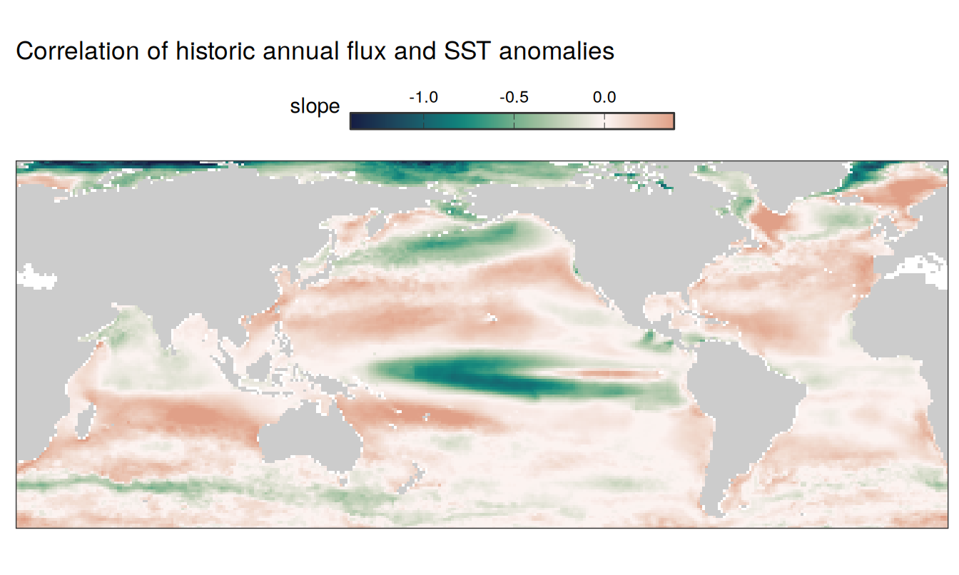

pco2_product_map_annual_anomaly_temperature_predict <-
  inner_join(
    pco2_product_map_annual_slope,
    pco2_product_map_annual_anomaly %>%
      filter(name %in% c("temperature", "fgco2")) %>% 
      select(lon, lat, name, resid, year) %>% 
      drop_na() %>% 
      arrange(desc(name)) %>% 
      pivot_wider(values_from = "resid")
  )

pco2_product_map_annual_anomaly_temperature_predict <-
  pco2_product_map_annual_anomaly_temperature_predict %>%
  mutate(fgco2_predict = slope * temperature)

pco2_product_map_annual_anomaly_temperature_predict %>%
  filter(year == 2023) %>%
  select(-slope) %>% 
  pivot_longer(c(fgco2, temperature, fgco2_predict),
               values_to = "resid") %>%
  drop_na() %>% 
  # filter(name == "fgco2_predict") %>% 
  group_split(name) %>% 
  # head(1) %>%
  map( ~ map +
         geom_tile(data = .x,
                   aes(lon, lat, fill = resid)) +
         labs(title =  paste(2023,"anomaly")) +
         scale_fill_gradientn(
           colours = cmocean("curl")(100),
           rescaler = ~ scales::rescale_mid(.x, mid = 0),
           name = labels_breaks(.x %>% distinct(name)),
           limits = c(quantile(.x$resid, .01), quantile(.x$resid, .99)),
           oob = squish
         ) +
      guides(
        fill = guide_colorbar(
          barheight = unit(0.3, "cm"),
          barwidth = unit(6, "cm"),
          ticks = TRUE,
          ticks.colour = "grey20",
          frame.colour = "grey20",
          label.position = "top",
          direction = "horizontal"
        )
      ) +
      theme(legend.title = element_markdown(),
            legend.position = "top")
  )

[[1]]

[[2]]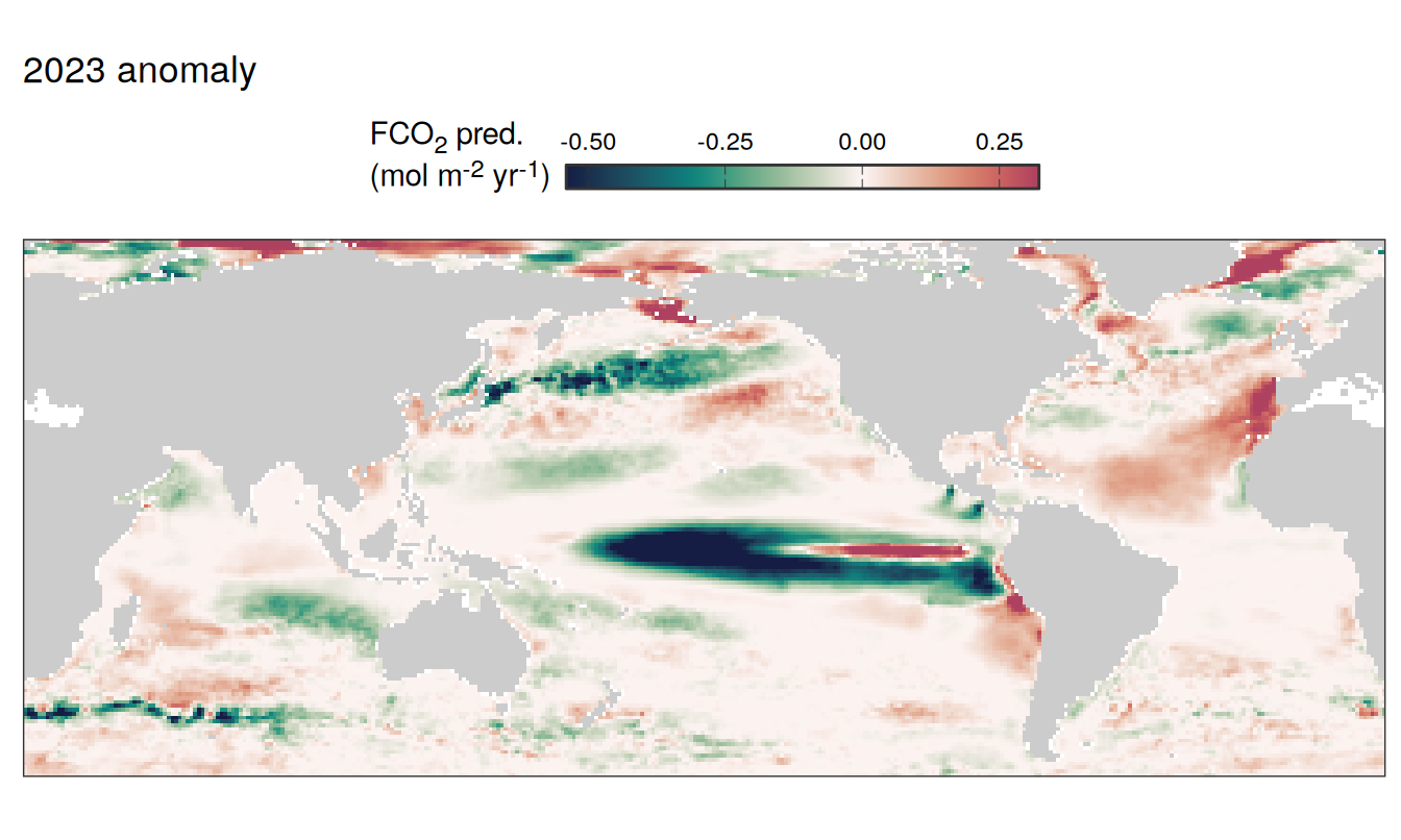

[[3]]

pco2_product_biome_annual_anomaly_temperature_predict <-
  full_join(
    pco2_product_map_annual_anomaly_temperature_predict %>% 
      select(lon, lat, year, temperature, fgco2, fgco2_predict),
    biome_mask %>%
      mutate(area = earth_surf(lat, lon))
  )


pco2_product_biome_annual_anomaly_temperature_predict_global <-
  pco2_product_biome_annual_anomaly_temperature_predict %>%
  drop_na() %>%
  mutate(fgco2_int = fgco2,
         fgco2_predict_int = fgco2_predict) %>%
  mutate(biome = case_when(str_detect(biome, "SO-SPSS|SO-ICE|Arctic") ~ "Polar",
                           TRUE ~ "Global non-polar")) %>%
  filter(biome == "Global non-polar") %>%
  select(-c(lon, lat)) %>%
  group_by(year, biome) %>%
  summarise(across(-c(fgco2_int, fgco2_predict_int, area),
                   ~ weighted.mean(., area, na.rm = TRUE)),
            across(c(fgco2_int, fgco2_predict_int),
                   ~ sum(. * area, na.rm = TRUE) * 12.01 * 1e-15)) %>%
  ungroup()

pco2_product_biome_annual_anomaly_temperature_predict <-
  pco2_product_biome_annual_anomaly_temperature_predict %>%
  drop_na() %>%
  mutate(fgco2_int = fgco2,
         fgco2_predict_int = fgco2_predict) %>%
  select(-c(lon, lat)) %>%
  group_by(year, biome) %>%
  summarise(across(-c(fgco2_int, fgco2_predict_int, area),
                   ~ weighted.mean(., area, na.rm = TRUE)),
            across(c(fgco2_int, fgco2_predict_int),
                   ~ sum(. * area, na.rm = TRUE) * 12.01 * 1e-15)) %>%
  ungroup()

pco2_product_biome_annual_anomaly_temperature_predict <-
  bind_rows(pco2_product_biome_annual_anomaly_temperature_predict_global,
            pco2_product_biome_annual_anomaly_temperature_predict)

rm(pco2_product_biome_annual_anomaly_temperature_predict_global)

pco2_product_biome_annual_anomaly_temperature_predict <-
  pco2_product_biome_annual_anomaly_temperature_predict %>% 
  filter(!is.na(biome))

pco2_product_biome_annual_anomaly_temperature_predict %>% 
  select(year, biome, fgco2_int, fgco2_predict_int) %>% 
  filter(biome == "Global non-polar") %>% 
  pivot_longer(starts_with("fgco2"),
               values_to = "resid") %>% 
  ggplot(aes(year, resid, col = name)) +
  geom_path() +
  geom_point()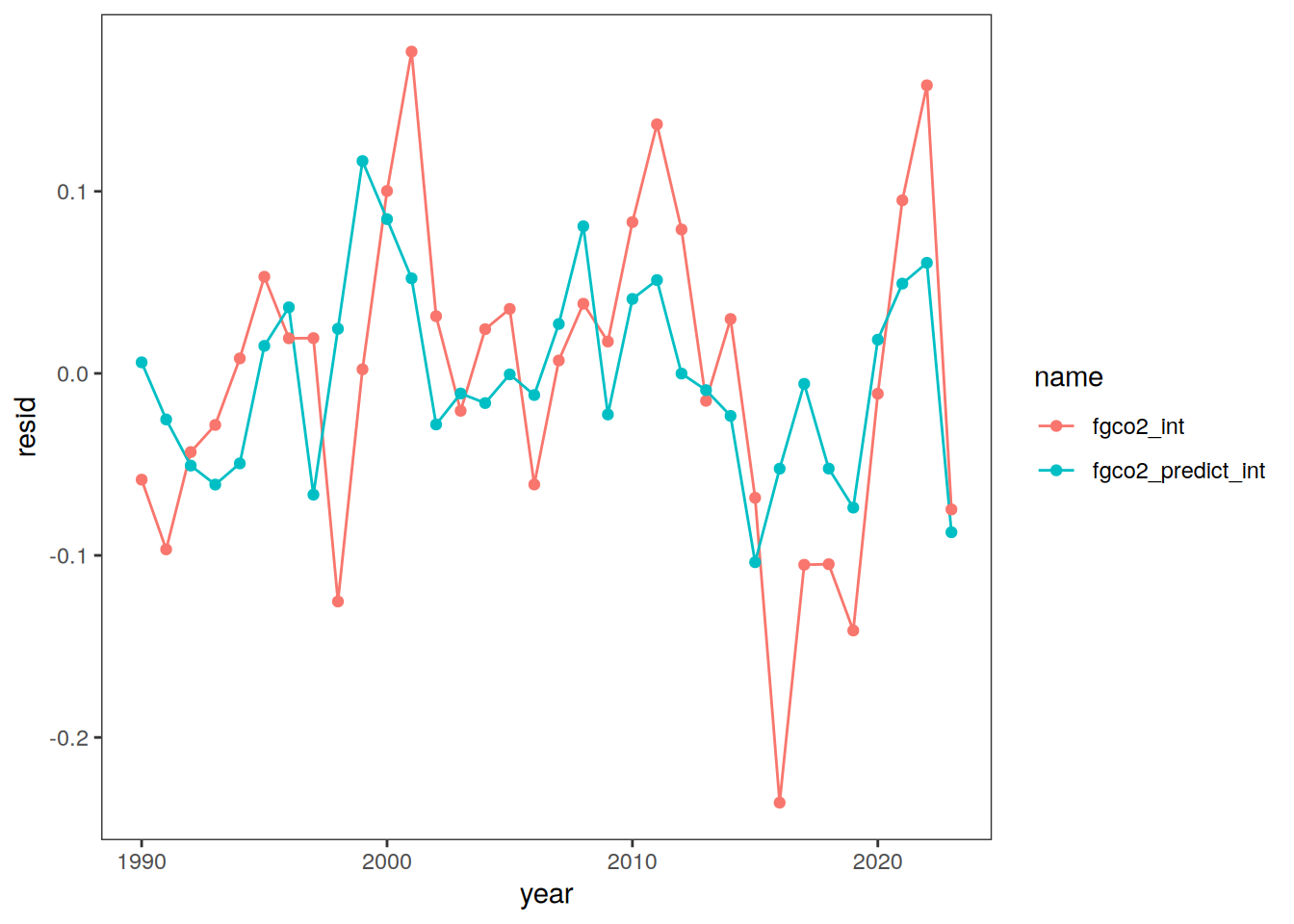

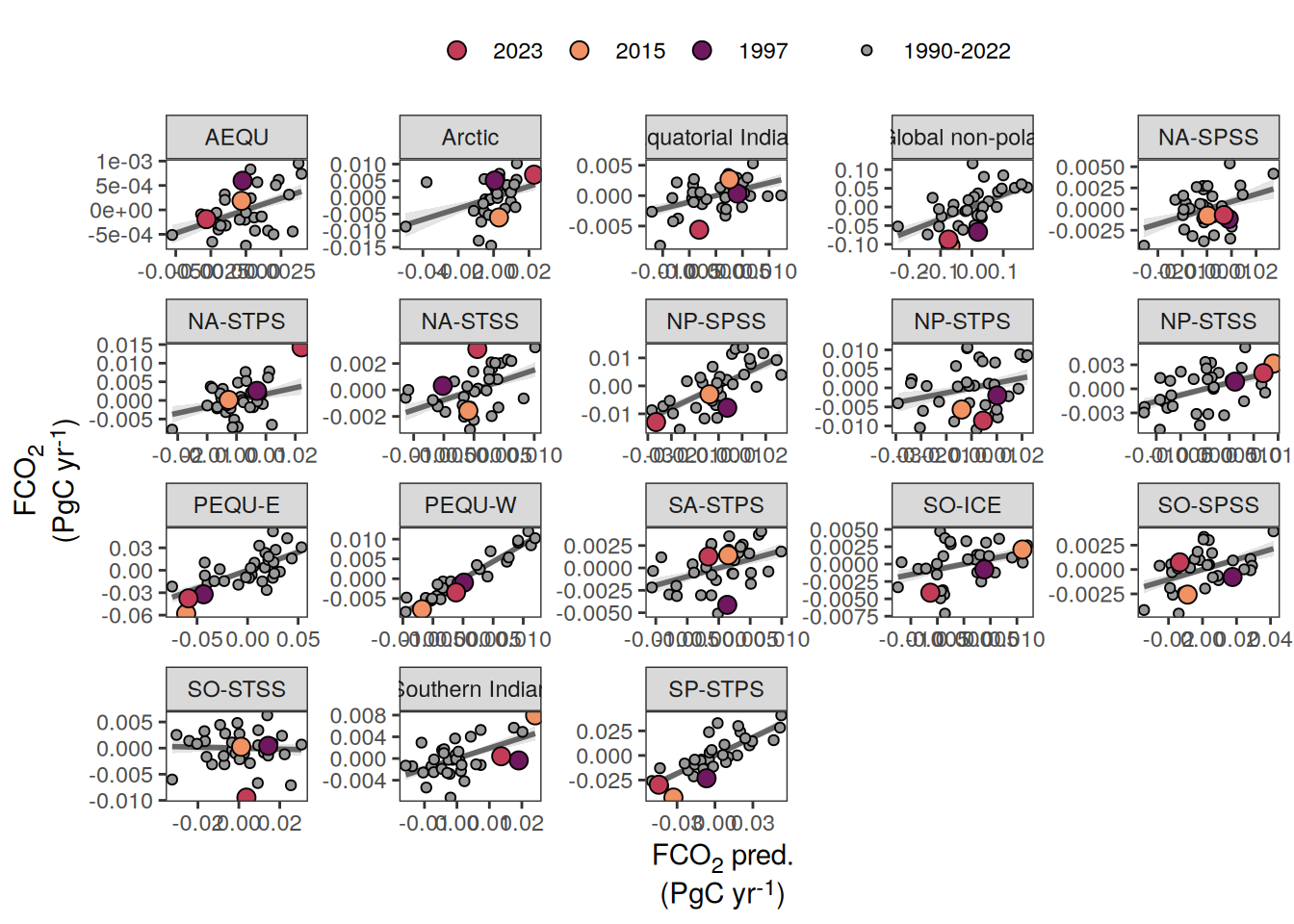
pco2_product_biome_annual_anomaly_temperature_predict %>%
  ggplot(aes(fgco2_int, fgco2_predict_int)) +
  geom_smooth(
    data = . %>% filter(year != 2023),
    method = "lm",
    fill = "grey",
    col = "grey40",
    fullrange = TRUE,
    level = 0.68
  ) +
  geom_point(data = . %>% filter(!year %in% c(2023, 1997, 2015)),
             aes(fill = "1990-2022"),
             shape = 21) +
  scale_color_manual(values = "grey60", name = "X") +
  scale_fill_manual(values = "grey60", name = "X") +
  new_scale_fill() +
  new_scale_color() +
  geom_point(
    data = . %>% filter(year %in% c(2023, 1997, 2015)),
    aes(fill = as.factor(year)),
    shape = 21,
    size = 3
  )  +
  scale_fill_manual(
    values = rev(warm_cool_gradient[c(17,13,20)]),
    guide = guide_legend(reverse = TRUE,
                         order = 2)
  ) +
  scale_color_manual(
    values = rev(warm_cool_gradient[c(17,13,20)]),
    guide = guide_legend(reverse = TRUE,
                         order = 2)
  ) +
  labs(y = labels_breaks("fgco2_int")$i_legend_title,
       x = labels_breaks("fgco2_predict_int")$i_legend_title) +
  facet_wrap(~ biome, scales = "free") +
  theme(
    axis.title.x = element_markdown(),
    axis.title.y = element_markdown(),
    legend.title = element_blank(),
    legend.position = "top"
  )

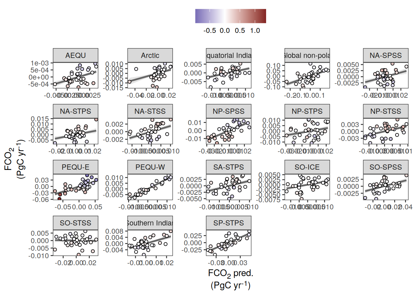
pco2_product_biome_annual_anomaly_temperature_predict %>%
  ggplot(aes(fgco2_int, fgco2_predict_int)) +
  geom_smooth(
    data = . %>% filter(year != 2023),
    method = "lm",
    fill = "grey",
    col = "grey40",
    fullrange = TRUE,
    level = 0.68
  ) +
  geom_point(aes(fill = temperature),
             shape = 21) +
  scale_fill_divergent() +
  labs(y = labels_breaks("fgco2_int")$i_legend_title,
       x = labels_breaks("fgco2_predict_int")$i_legend_title) +
  facet_wrap(~ biome, scales = "free") +
  theme(
    axis.title.x = element_markdown(),
    axis.title.y = element_markdown(),
    legend.title = element_blank(),
    legend.position = "top"
  )

pco2_product_map_annual_anomaly %>%
  filter(year == 2023) %>%
  write_csv(
    paste0(
      "../data/",
      "NIES-ML3_GCB",
      "_",
      "2023",
      "_map_annual_anomaly.csv"
    )
  )

pco2_product_map_annual_anomaly_temperature_predict %>%
  filter(year == 2023) %>%
  write_csv(
    paste0(
      "../data/",
      "NIES-ML3_GCB",
      "_",
      "2023",
      "_map_annual_anomaly_temperature_predict.csv"
    )
  )

pco2_product_biome_annual_anomaly_temperature_predict %>%
  write_csv(
    paste0(
      "../data/",
      "NIES-ML3_GCB",
      "_",
      "2023",
      "_biome_annual_anomaly_temperature_predict.csv"
    )
  )

rm(pco2_product_map_annual_anomaly,
   pco2_product_map_annual_slope,
   pco2_product_map_annual_anomaly_temperature_predict,
   pco2_product_biome_annual_anomaly_temperature_predict)
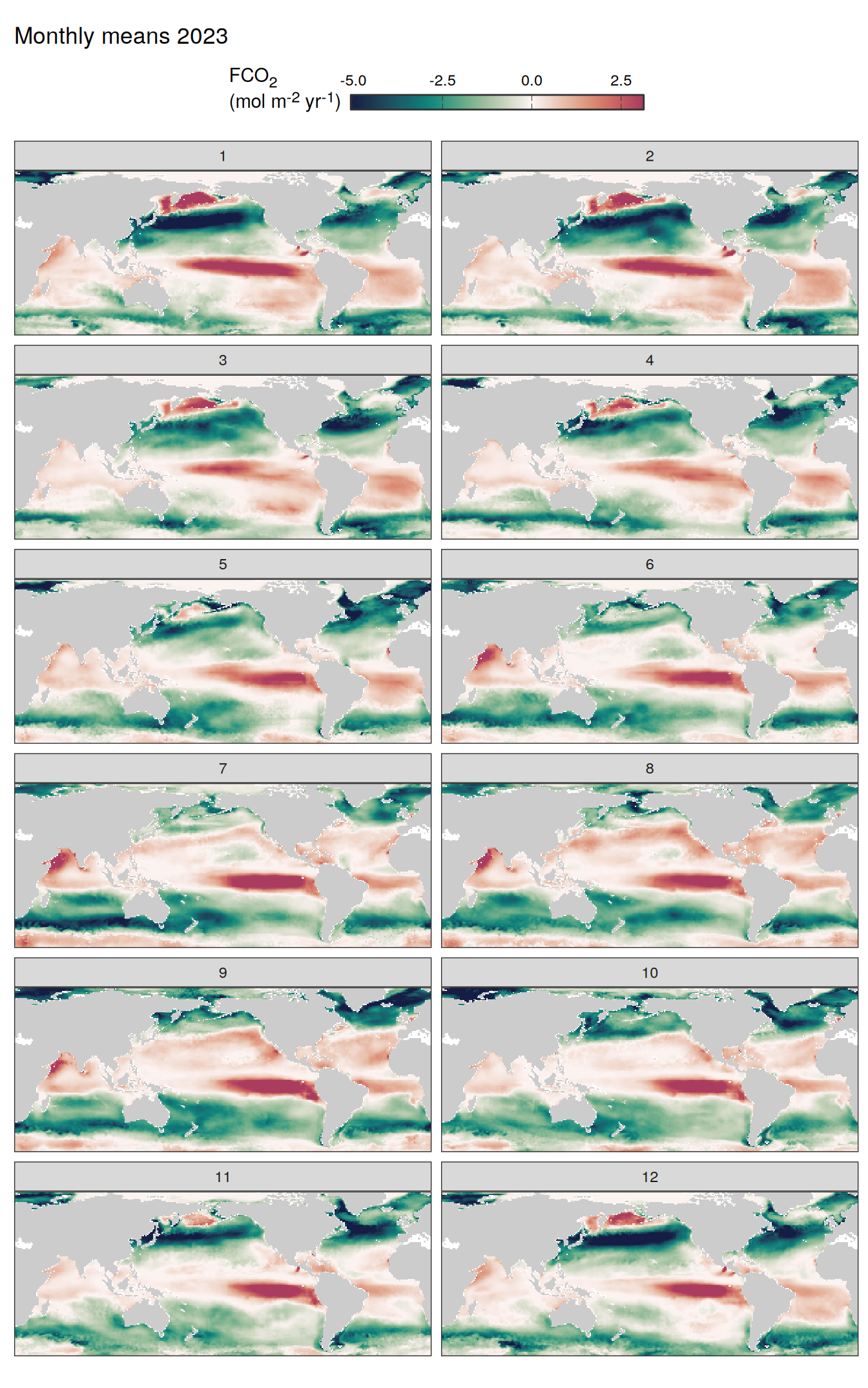
gc()

Monthly means

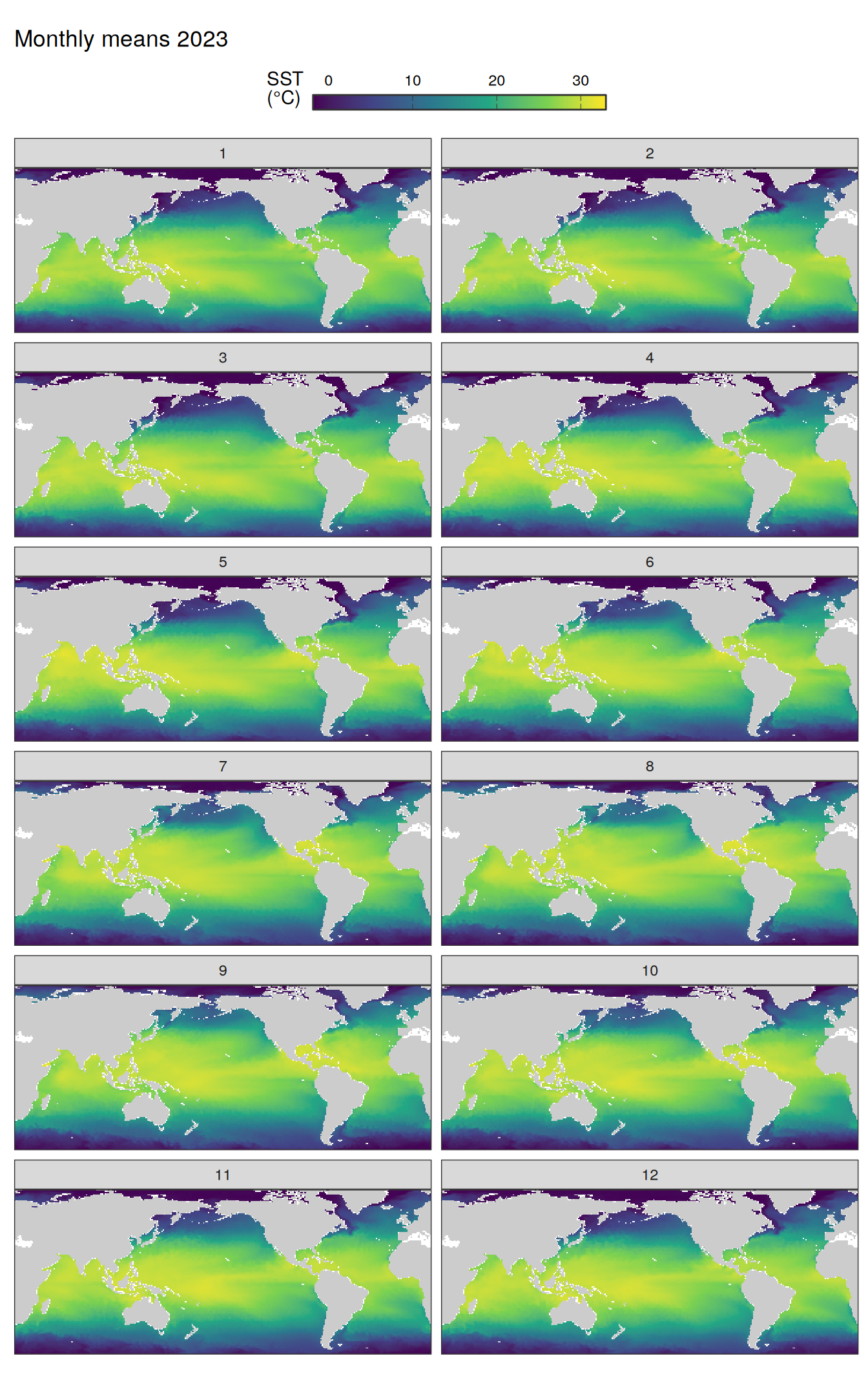
2023 absolute

pco2_product_map_monthly_anomaly <-
  pco2_product_map_monthly %>%
  drop_na() %>% 
  anomaly_determination(lon, lat, month)

pco2_product_map_monthly_anomaly <-
  pco2_product_map_monthly_anomaly %>% 
  drop_na()



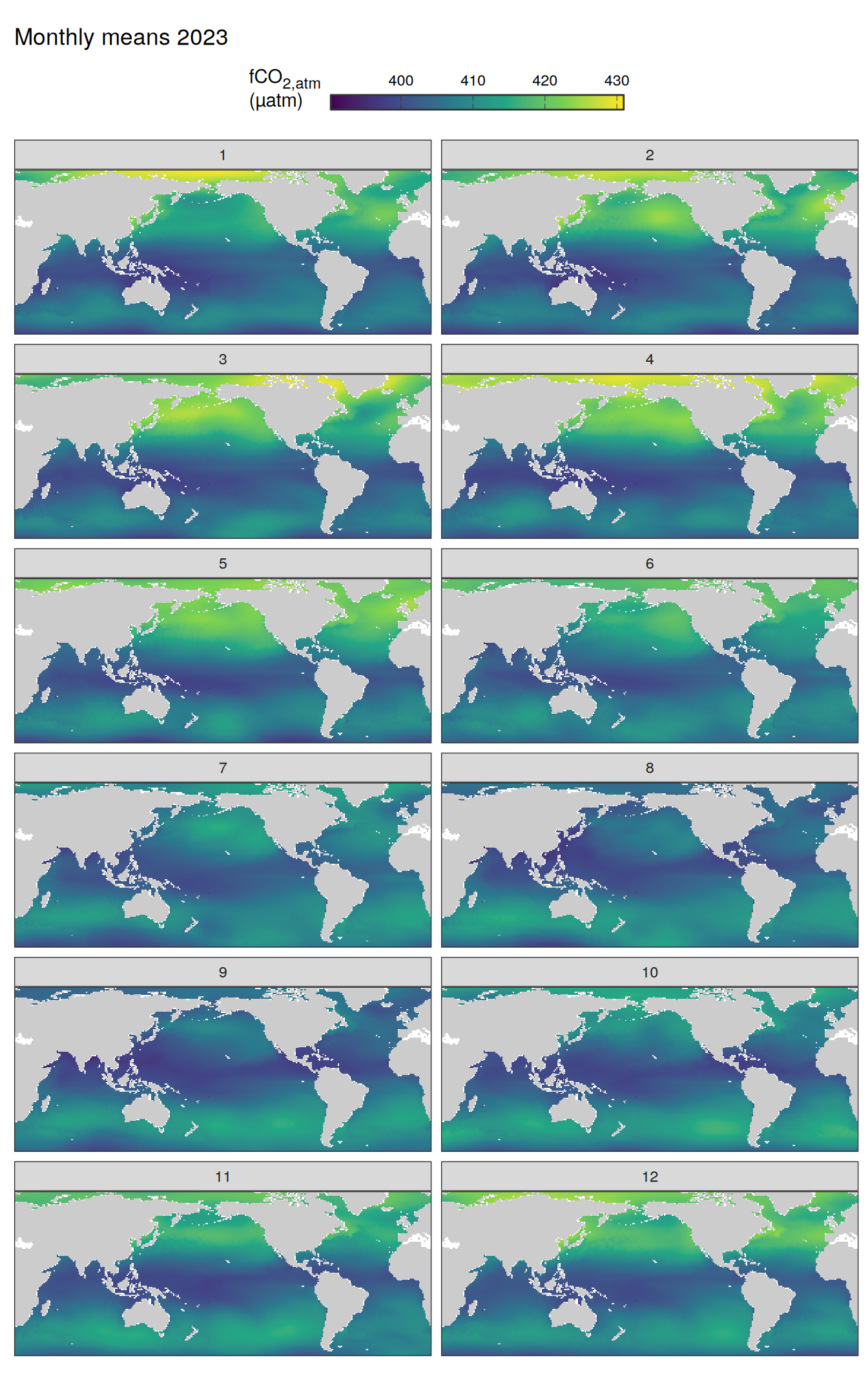
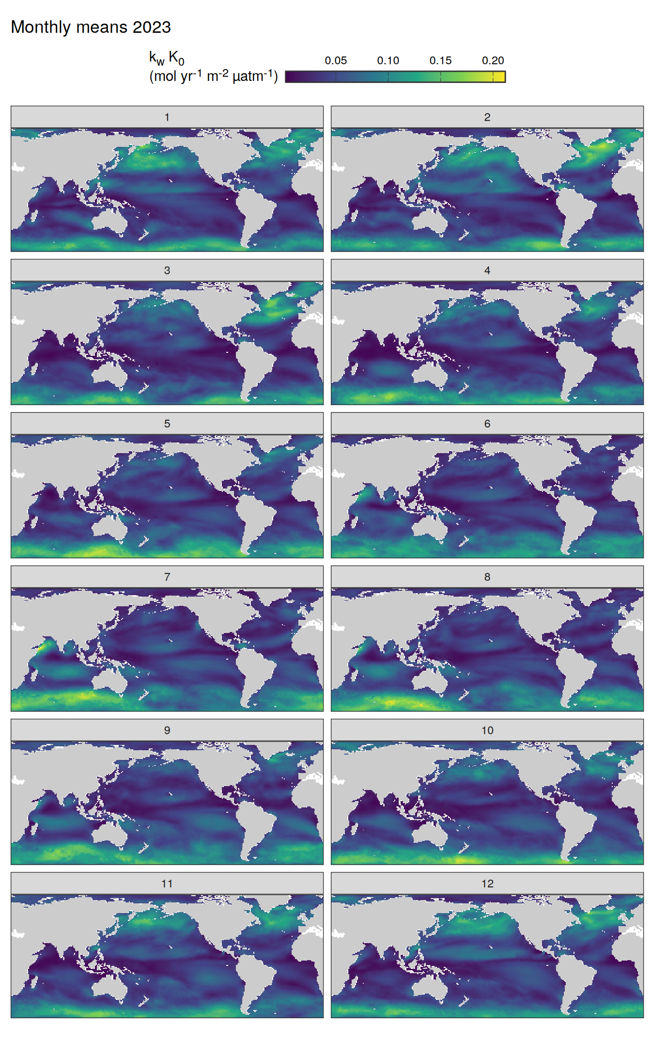
pco2_product_map_monthly_anomaly %>%
  filter(year == 2023, !(name %in% name_divergent)) %>%
  group_split(name) %>%
  # head(1) %>%
  map(
    ~ map +
      geom_tile(data = .x, aes(lon, lat, fill = value)) +
      labs(title = paste("Monthly means", 2023)) +
      scale_fill_viridis_c(name = labels_breaks(.x %>% distinct(name))) +
      guides(
        fill = guide_colorbar(
          barheight = unit(0.3, "cm"),
          barwidth = unit(6, "cm"),
          ticks = TRUE,
          ticks.colour = "grey20",
          frame.colour = "grey20",
          label.position = "top",
          direction = "horizontal"
        )
      ) +
      theme(legend.title = element_markdown(), legend.position = "top") +
      facet_wrap(~ month, ncol = 2)
  )

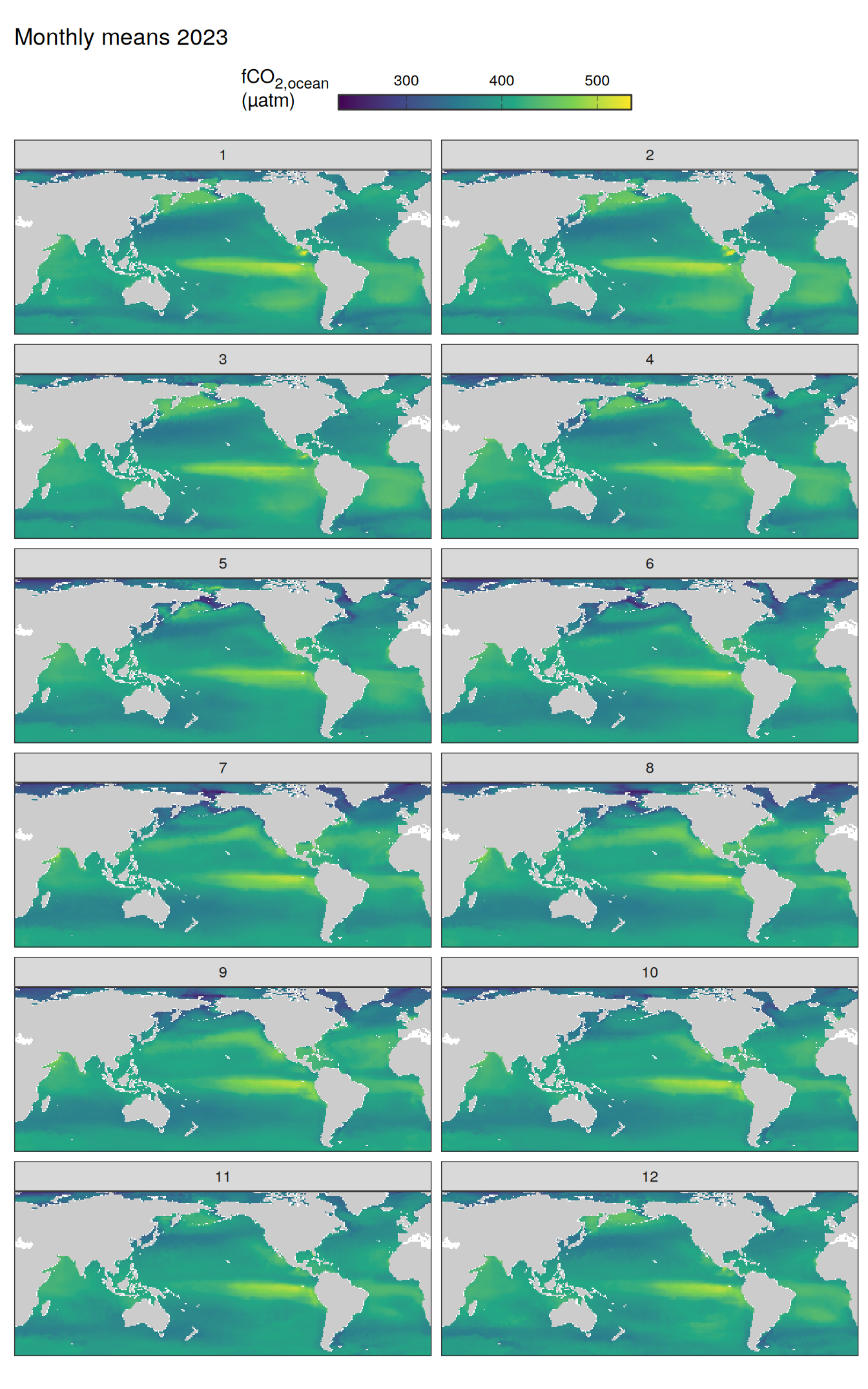
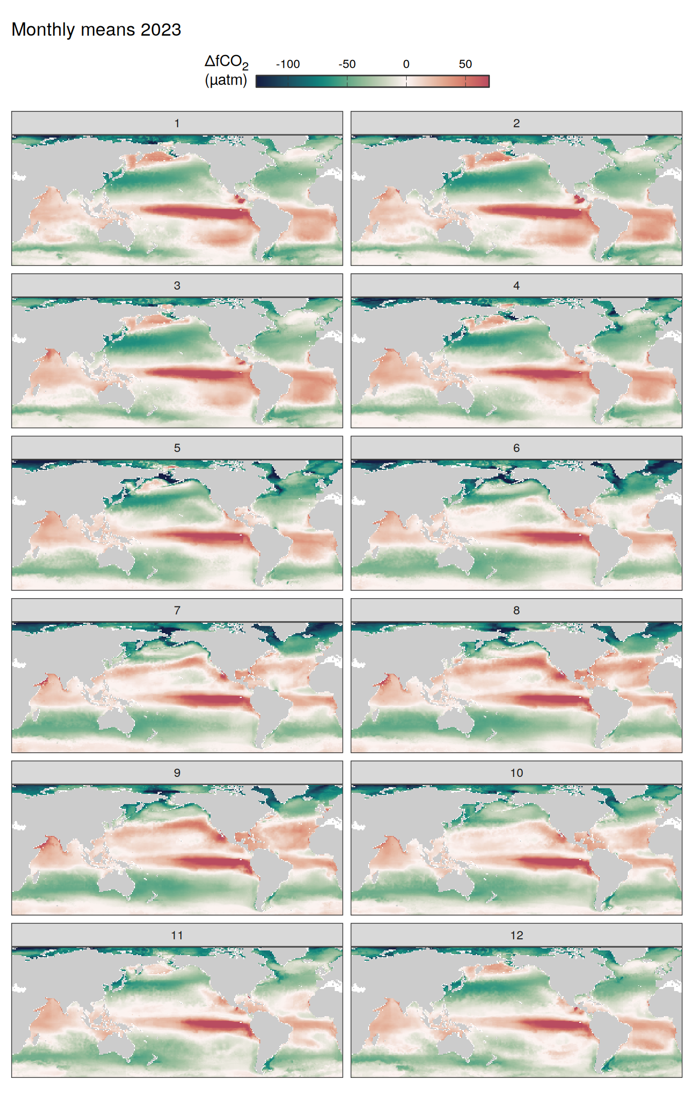
pco2_product_map_monthly_anomaly %>%
  filter(year == 2023, name %in% name_divergent) %>%
  group_split(name) %>%
  # head(1) %>%
  map(
    ~ map +
      geom_tile(data = .x, aes(lon, lat, fill = value)) +
      labs(title = paste("Monthly means", 2023)) +
      scale_fill_gradientn(
        colours = cmocean("curl")(100),
        rescaler = ~ scales::rescale_mid(.x, mid = 0),
        name = labels_breaks(.x %>% distinct(name)),
        limits = c(quantile(.x$value, .01), quantile(.x$value, .99)),
        oob = squish
      ) +
      guides(
        fill = guide_colorbar(
          barheight = unit(0.3, "cm"),
          barwidth = unit(6, "cm"),
          ticks = TRUE,
          ticks.colour = "grey20",
          frame.colour = "grey20",
          label.position = "top",
          direction = "horizontal"
        )
      ) +
      theme(legend.title = element_markdown(), legend.position = "top") +
      facet_wrap( ~ month, ncol = 2)
  )

Trends

pco2_product_map_monthly_anomaly %>%
  group_by(name) %>%
  filter(year %in% c(min(year), max(year))) %>%
  ungroup() %>%
  select(-c(value, resid)) %>%
  arrange(year) %>%
  group_by(lon, lat, name, month) %>%
  mutate(change = fit - lag(fit),
         period = paste(lag(year), year, sep = "-")) %>%
  ungroup() %>%
  filter(!is.na(change)) %>%
  group_split(name) %>%
  head(1) %>%
  map(
    ~ map +
      geom_tile(data = .x, aes(lon, lat, fill = change)) +
      labs(title =  paste("Change: ", .x$period)) +
      scale_fill_gradientn(
        colours = cmocean("curl")(100),
        rescaler = ~ scales::rescale_mid(.x, mid = 0),
        name = labels_breaks(.x %>% distinct(name)),
        limits = c(quantile(.x$change, .01), quantile(.x$change, .99)),
        oob = squish
      ) +
      guides(
        fill = guide_colorbar(
          barheight = unit(0.3, "cm"),
          barwidth = unit(6, "cm"),
          ticks = TRUE,
          ticks.colour = "grey20",
          frame.colour = "grey20",
          label.position = "top",
          direction = "horizontal"
        )
      ) +
      theme(legend.title = element_markdown(), legend.position = "top") +
      facet_wrap(~ month, ncol = 2)
  )

2023 anomaly

pco2_product_map_monthly_anomaly %>%
  filter(year == 2023) %>%
  group_split(name) %>%
  # head(1) %>%
  map(
    ~ map +
      geom_tile(data = .x, aes(lon, lat, fill = resid)) +
      labs(title = paste(2023, "anomaly")) +
      scale_fill_gradientn(
        colours = cmocean("curl")(100),
        rescaler = ~ scales::rescale_mid(.x, mid = 0),
        name = labels_breaks(.x %>% distinct(name)),
        limits = c(quantile(.x$resid, .01), quantile(.x$resid, .99)),
        oob = squish
      ) +
      guides(
        fill = guide_colorbar(
          barheight = unit(0.3, "cm"),
          barwidth = unit(6, "cm"),
          ticks = TRUE,
          ticks.colour = "grey20",
          frame.colour = "grey20",
          label.position = "top",
          direction = "horizontal"
        )
      ) +
      theme(legend.title = element_markdown(), legend.position = "top") +
      facet_wrap( ~ month, ncol = 2)
  )

fCO2 decomposition

pco2_product_map_monthly_fCO2_decomposition <-
  fco2_decomposition(pco2_product_map_monthly_anomaly,
                     year, month, lon, lat)


# pco2_product_map_monthly_fCO2_decomposition %>%
#   filter(year == 2023) %>%
#   mutate(product == "pco2 product") %>%
#   group_split(product) %>%
#   head(1) %>%
#   map(
#     ~ map +
#       geom_tile(data = .x,
#                 aes(lon, lat, fill = resid)) +
#       labs(title = .x$product) +
#       scale_fill_gradientn(
#         colours = cmocean("curl")(100),
#         rescaler = ~ scales::rescale_mid(.x, mid = 0),
#         name = labels_breaks("sfco2"),
#         limits = c(quantile(.x$resid, .01), quantile(.x$resid, .99)),
#         oob = squish
#       ) +
#       facet_grid(month ~ name,
#                  labeller = labeller(name = x_axis_labels)) +
#       guides(
#         fill = guide_colorbar(
#           barheight = unit(0.3, "cm"),
#           barwidth = unit(6, "cm"),
#           ticks = TRUE,
#           ticks.colour = "grey20",
#           frame.colour = "grey20",
#           label.position = "top",
#           direction = "horizontal"
#         )
#       ) +
#       theme(legend.title = element_markdown(),
#             legend.position = "top")
#   )

pco2_product_map_annual_fCO2_decomposition <-
  pco2_product_map_monthly_fCO2_decomposition %>% 
  select(year, lat, lon, name, resid) %>% 
  fgroup_by(year, lat, lon, name) %>% 
  fmean()

gc()

             used    (Mb) gc trigger    (Mb)   max used    (Mb)
Ncells    4291288   229.2   27299156  1458.0  104138011  5561.6
Vcells 1683142661 12841.4 3844364568 29330.2 3844324302 29329.9

map +
  geom_tile(data = pco2_product_map_annual_fCO2_decomposition %>%
              filter(year == 2023), aes(lon, lat, fill = resid)) +
  scale_fill_gradientn(
    colours = cmocean("curl")(100),
    rescaler = ~ scales::rescale_mid(.x, mid = 0),
    name = labels_breaks("sfco2"),
    limits = c(
      quantile(pco2_product_map_annual_fCO2_decomposition$resid, .01),
      quantile(pco2_product_map_annual_fCO2_decomposition$resid, .99)
    ),
    oob = squish
  ) +
  facet_wrap(~ name,
             ncol = 2,
             labeller = labeller(name = x_axis_labels)) +
  guides(
    fill = guide_colorbar(
      barheight = unit(0.3, "cm"),
      barwidth = unit(6, "cm"),
      ticks = TRUE,
      ticks.colour = "grey20",
      frame.colour = "grey20",
      label.position = "top",
      direction = "horizontal"
    )
  ) +
  theme(legend.title = element_markdown(), legend.position = "top")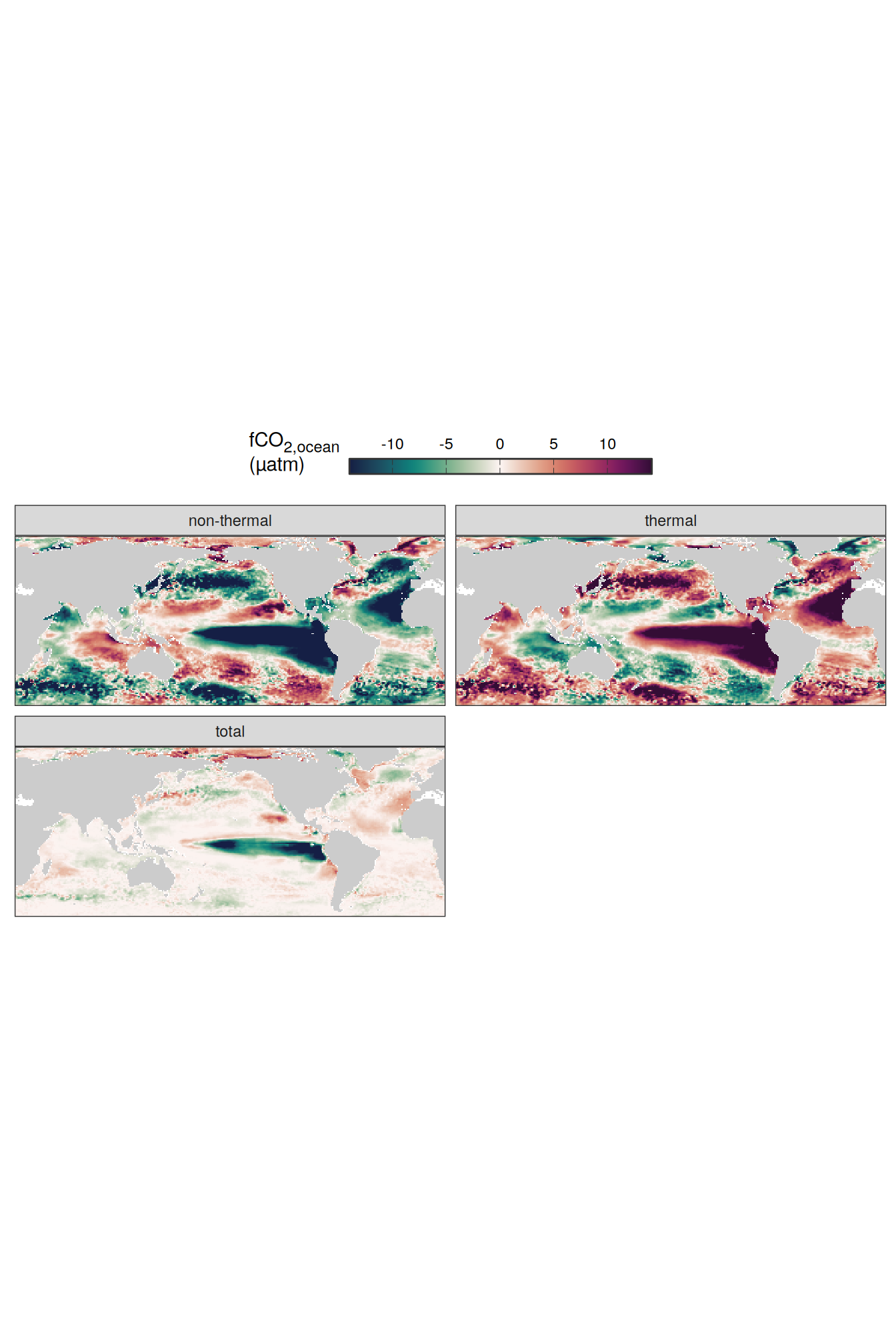

Flux attribution

pco2_product_map_monthly_flux_attribution <-
  flux_attribution(pco2_product_map_monthly_anomaly,
                   year, month, lon, lat)

# pco2_product_map_monthly_flux_attribution %>%
#   filter(year == 2023) %>%
#   drop_na() %>%
#   mutate(product == "pco2 product") %>%
#   group_split(product) %>%
#   head(1) %>%
#   map(
#     ~ map +
#       geom_tile(data = .x,
#                 aes(lon, lat, fill = resid)) +
#       labs(subtitle = .x$product) +
#       scale_fill_gradientn(
#         colours = cmocean("curl")(100),
#         rescaler = ~ scales::rescale_mid(.x, mid = 0),
#         name = labels_breaks("fgco2"),
#         limits = c(quantile(.x$resid, .01), quantile(.x$resid, .99)),
#         oob = squish
#       ) +
#       theme(legend.title = element_markdown(),
#             legend.position = "bottom") +
#       facet_grid(month ~ name,
#                  labeller = labeller(name = x_axis_labels)) +
#       guides(
#         fill = guide_colorbar(
#           barheight = unit(0.3, "cm"),
#           barwidth = unit(6, "cm"),
#           ticks = TRUE,
#           ticks.colour = "grey20",
#           frame.colour = "grey20",
#           label.position = "top",
#           direction = "horizontal"
#         )
#       ) +
#       theme(legend.title = element_markdown(),
#             legend.position = "top",
#             strip.text.x.top = element_markdown())
#   )

pco2_product_map_annual_flux_attribution <-
  pco2_product_map_monthly_flux_attribution %>% 
  group_by(year, lat, lon, name) %>% 
  summarise(resid = mean(resid, na.rm = TRUE)) %>% 
  ungroup()

map +
  geom_tile(data = pco2_product_map_annual_flux_attribution %>%
              filter(year == 2023), aes(lon, lat, fill = resid)) +
  scale_fill_gradientn(
    colours = cmocean("curl")(100),
    rescaler = ~ scales::rescale_mid(.x, mid = 0),
    name = labels_breaks("fgco2"),
    limits = c(
      quantile(pco2_product_map_annual_flux_attribution$resid, .01, na.rm = TRUE),
      quantile(pco2_product_map_annual_flux_attribution$resid, .99, na.rm = TRUE)
    ),
    oob = squish
  ) +
  theme(legend.title = element_markdown(), legend.position = "bottom") +
  facet_wrap(~ name,
             ncol = 2,
             labeller = labeller(name = x_axis_labels)) +
  guides(
    fill = guide_colorbar(
      barheight = unit(0.3, "cm"),
      barwidth = unit(6, "cm"),
      ticks = TRUE,
      ticks.colour = "grey20",
      frame.colour = "grey20",
      label.position = "top",
      direction = "horizontal"
    )
  ) +
  theme(
    legend.title = element_markdown(),
    legend.position = "top",
    strip.text.x.top = element_markdown()
    
  )

gc()

             used    (Mb) gc trigger    (Mb)   max used    (Mb)
Ncells    4309498   230.2   21839325  1166.4  104138011  5561.6
Vcells 1938693021 14791.1 3844364568 29330.2 3844324302 29329.9

pco2_product_map_monthly_anomaly %>%
  filter(year == 2023) %>%
  write_csv(
    paste0(
      "../data/",
      "NIES-ML3_GCB",
      "_",
      "2023",
      "_map_monthly_anomaly.csv"
    )
  )

pco2_product_map_annual_flux_attribution %>%
  filter(year == 2023) %>%
  write_csv(
    paste0(
      "../data/",
      "NIES-ML3_GCB",
      "_",
      "2023",
      "_map_annual_flux_attribution.csv"
    )
  )

pco2_product_map_annual_fCO2_decomposition %>%
  filter(year == 2023) %>%
  write_csv(
    paste0(
      "../data/",
      "NIES-ML3_GCB",
      "_",
      "2023",
      "_map_annual_fCO2_decomposition.csv"
    )
  )

pco2_product_map_monthly_flux_attribution %>%
  filter(year == 2023) %>%
  write_csv(
    paste0(
      "../data/",
      "NIES-ML3_GCB",
      "_",
      "2023",
      "_map_monthly_flux_attribution.csv"
    )
  )

pco2_product_map_monthly_fCO2_decomposition %>%
  filter(year == 2023) %>%
  write_csv(
    paste0(
      "../data/",
      "NIES-ML3_GCB",
      "_",
      "2023",
      "_map_monthly_fCO2_decomposition.csv"
    )
  )

rm(pco2_product_map_annual_flux_attribution,
   pco2_product_map_annual_fCO2_decomposition)

gc()

Hovmoeller plots

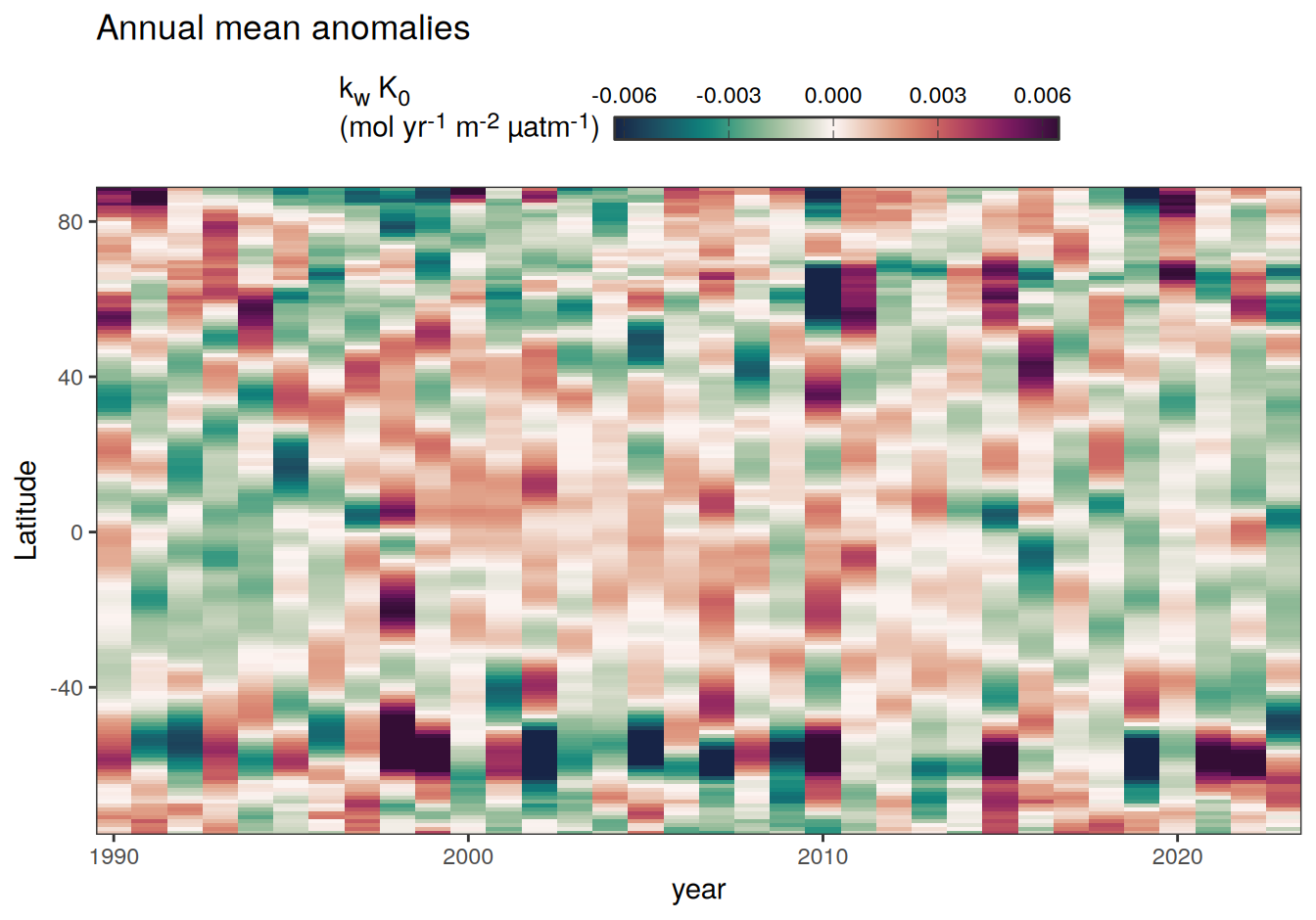
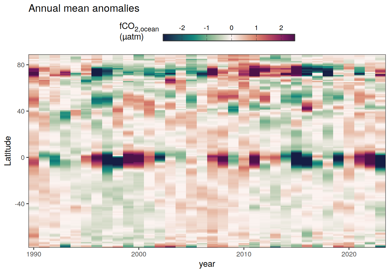
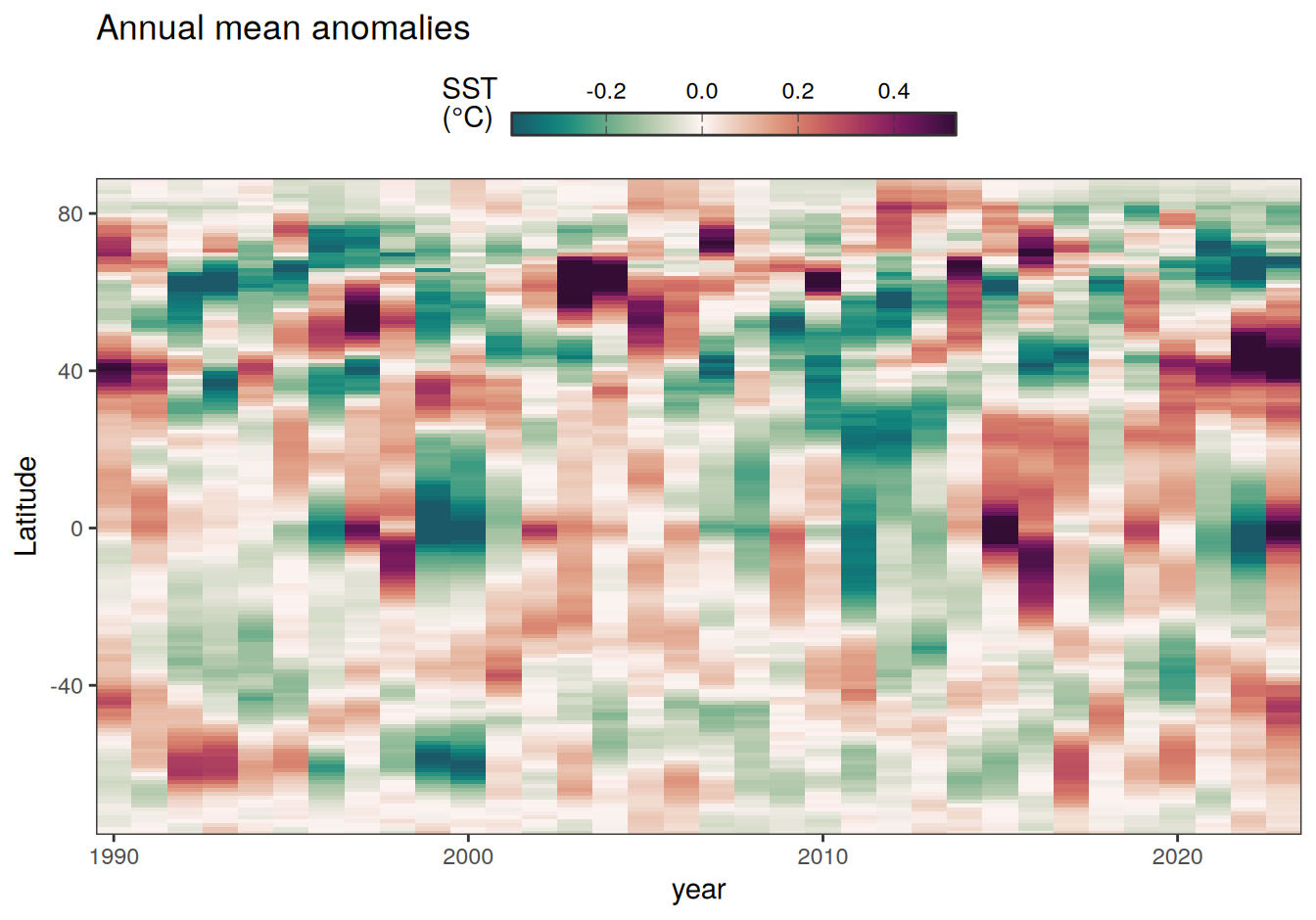
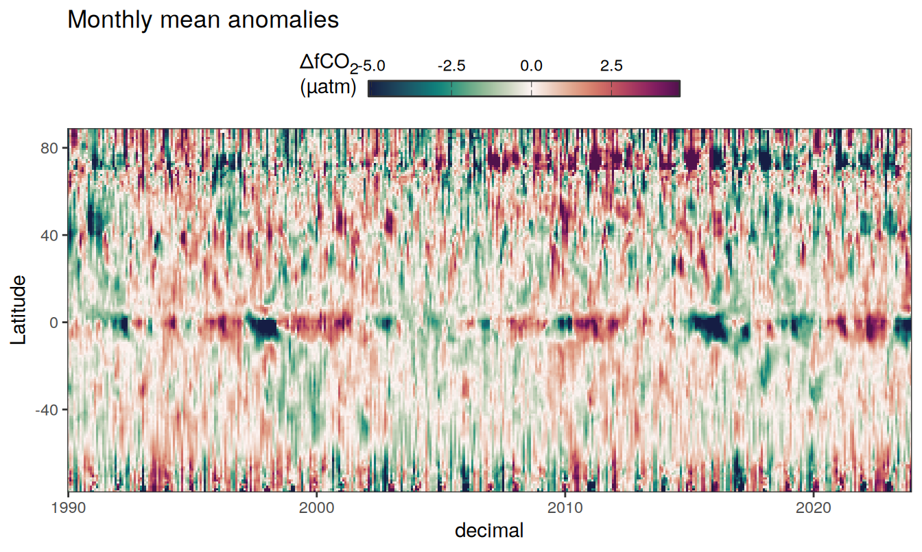
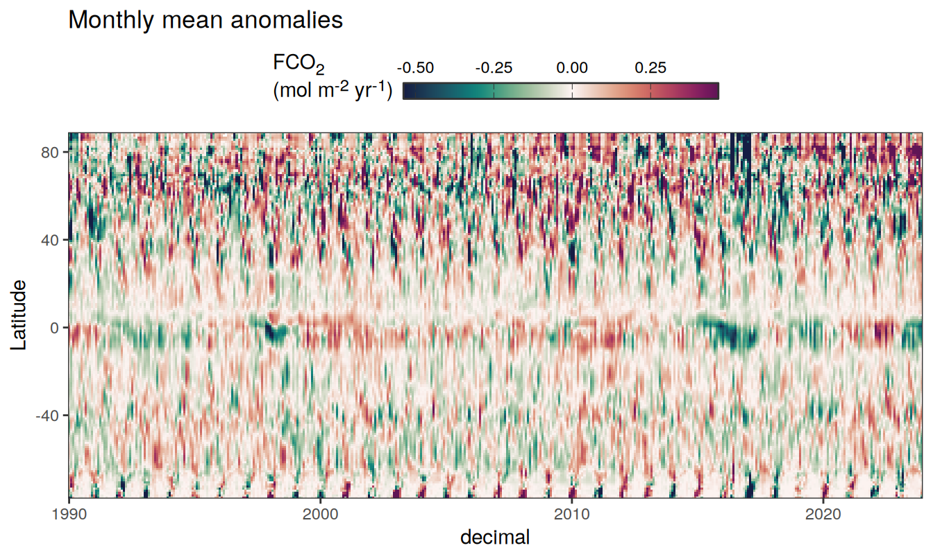
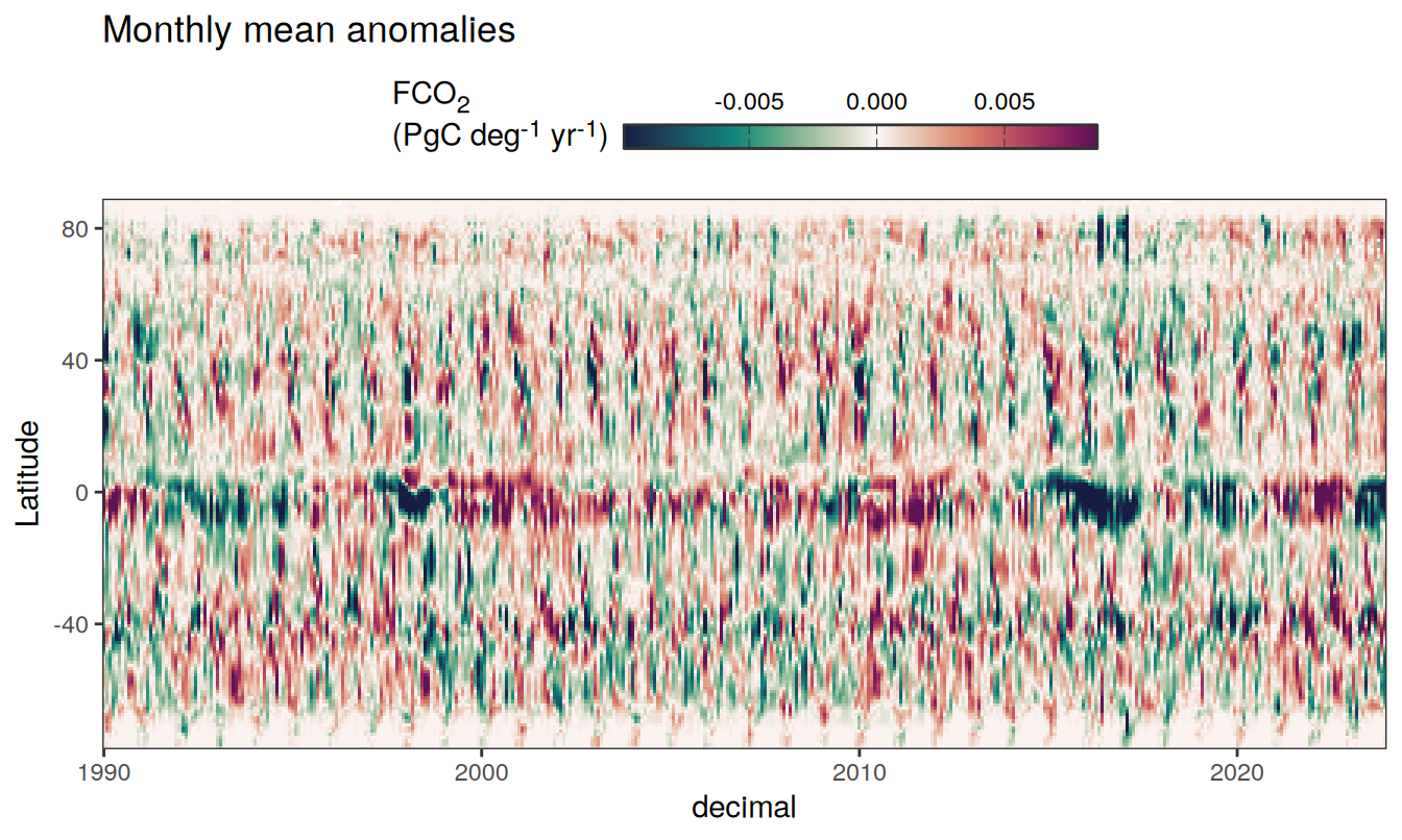
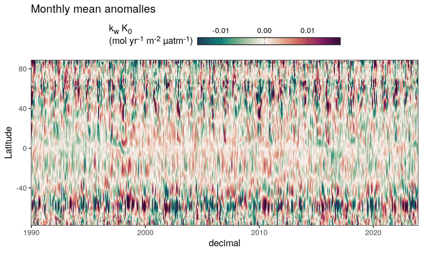
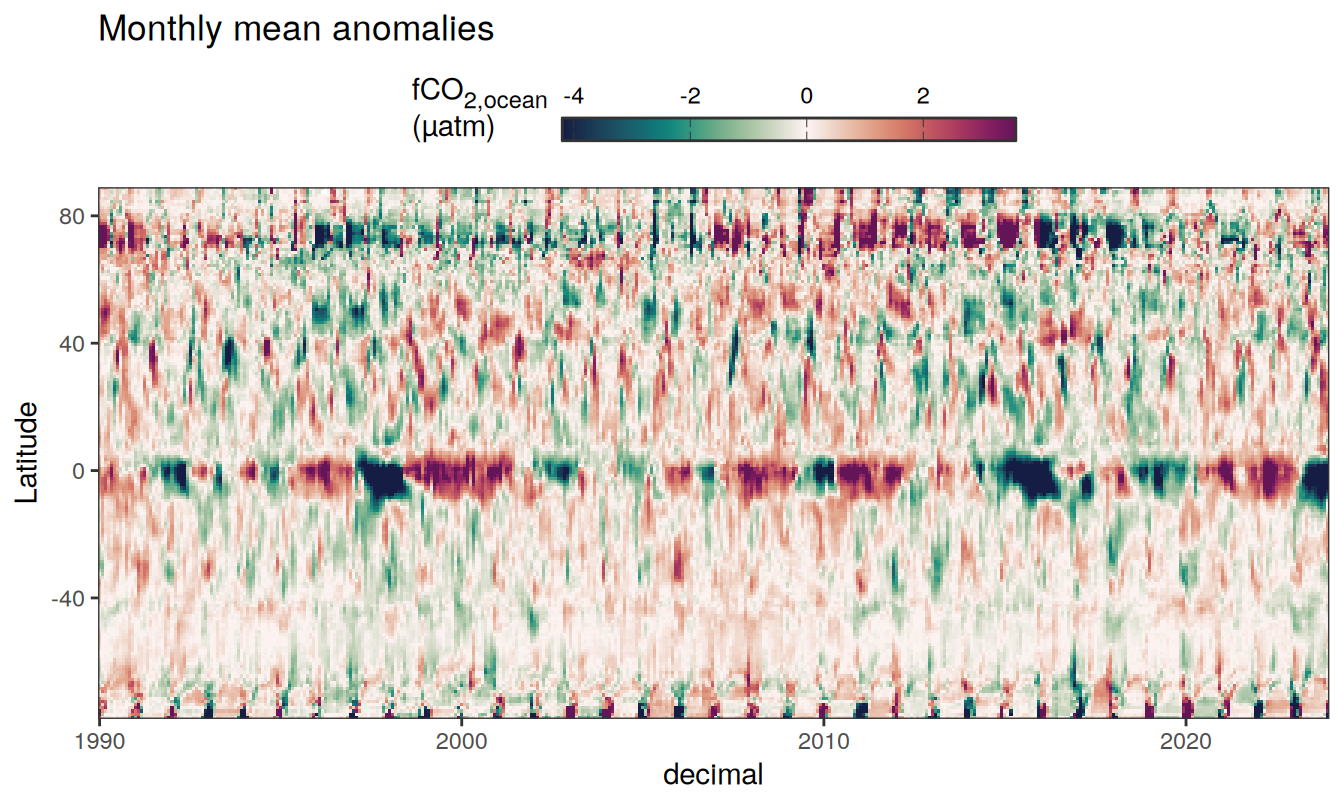
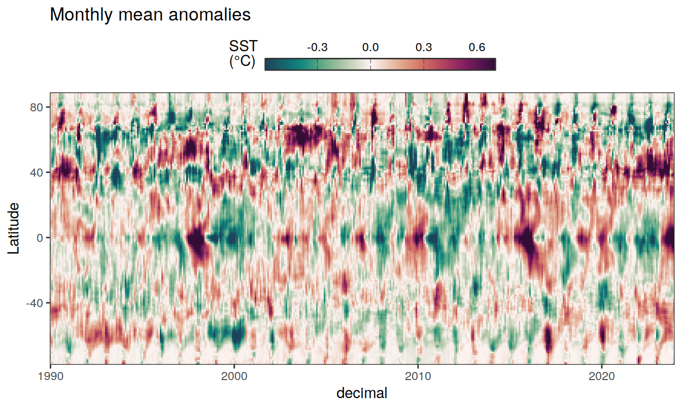
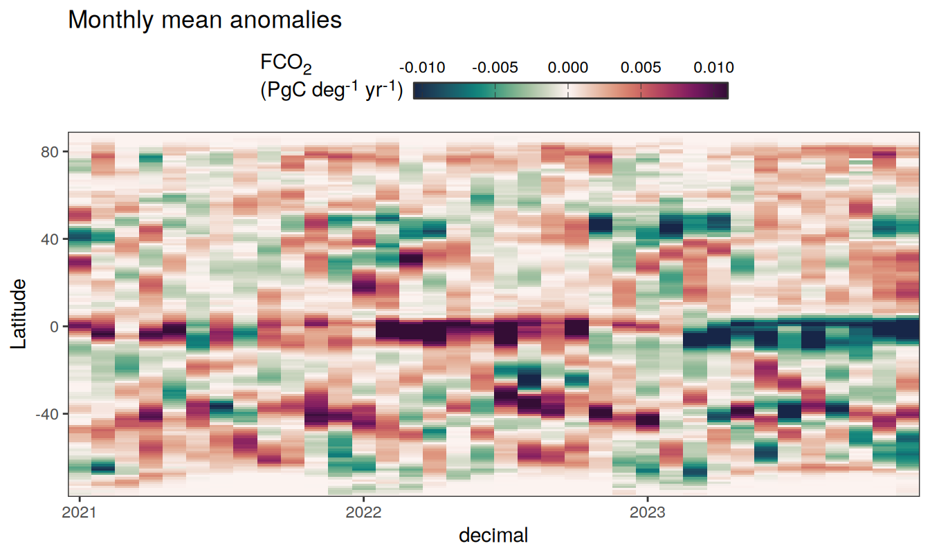
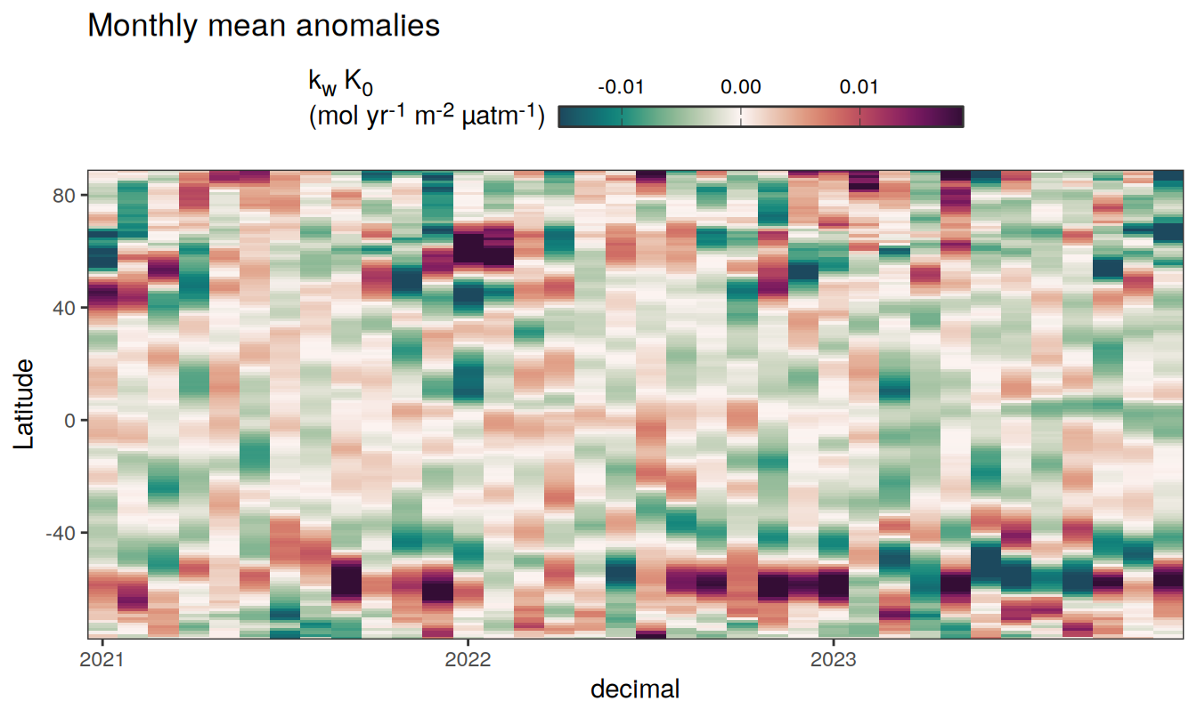
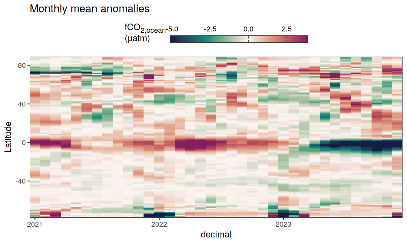
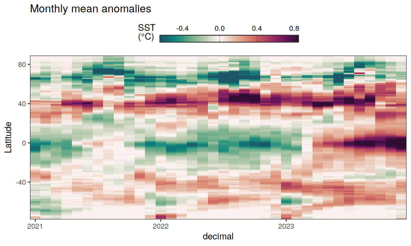
The following Hovmoeller plots show the anomalies from the prediction of the linear/quadratic fits.

Hovmoeller plots are first presented as annual means, and than as monthly means. Note that the predictions for the monthly Hovmoeller plots are done individually for each month, such the mean seasonal anomaly from the annual mean is removed.

2023 annual anomalies

pco2_product_hovmoeller_annual_anomaly <-
  pco2_product_hovmoeller_annual %>%
  anomaly_determination(lat) %>% 
  filter(!is.na(resid))

  
pco2_product_hovmoeller_annual_anomaly %>%
  # filter(name == "mld") %>%
  group_split(name) %>%
  # head(1) %>%
  map(
    ~ ggplot(data = .x, aes(year, lat, fill = resid)) +
      geom_raster() +
      scale_fill_gradientn(
        colours = cmocean("curl")(100),
        rescaler = ~ scales::rescale_mid(.x, mid = 0),
        name = labels_breaks(.x %>% distinct(name)),
        limits = c(quantile(.x$resid, .01), quantile(.x$resid, .99)),
        oob = squish
      ) +
      coord_cartesian(expand = 0) +
      labs(title = "Annual mean anomalies", y = "Latitude") +
      guides(
        fill = guide_colorbar(
          barheight = unit(0.3, "cm"),
          barwidth = unit(6, "cm"),
          ticks = TRUE,
          ticks.colour = "grey20",
          frame.colour = "grey20",
          label.position = "top",
          direction = "horizontal"
        )
      ) +
      theme(legend.title = element_markdown(), legend.position = "top")
  )

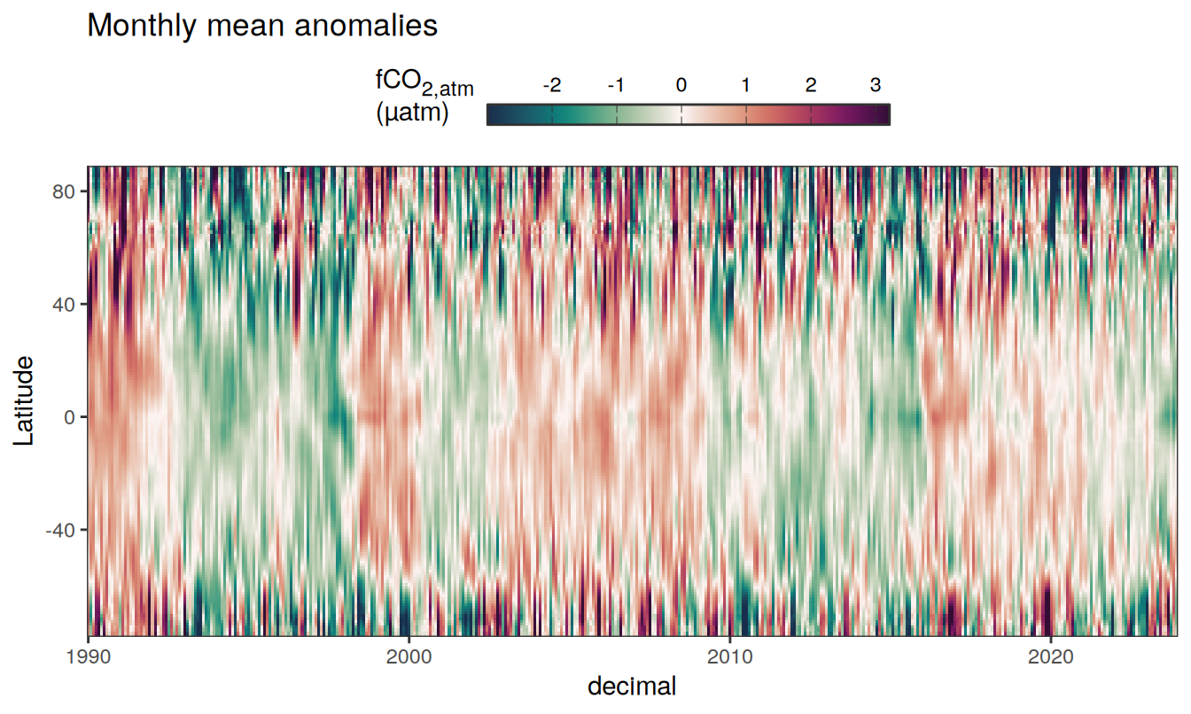
2023 monthly anomalies

pco2_product_hovmoeller_monthly_anomaly <-
  pco2_product_hovmoeller_monthly %>%
  select(-c(decimal)) %>% 
  anomaly_determination(lat, month) %>% 
  filter(!is.na(resid))

  
pco2_product_hovmoeller_monthly_anomaly <-
  pco2_product_hovmoeller_monthly_anomaly %>%
  mutate(decimal = year + (month - 1) / 12)
  
pco2_product_hovmoeller_monthly_anomaly %>%
  group_split(name) %>%
  # head(1) %>%
  map(
    ~ ggplot(data = .x,
             aes(decimal, lat, fill = resid)) +
      geom_raster() +
      scale_fill_gradientn(
        colours = cmocean("curl")(100),
        rescaler = ~ scales::rescale_mid(.x, mid = 0),
        name = labels_breaks(.x %>% distinct(name)),
        limits = c(quantile(.x$resid, .01), quantile(.x$resid, .99)),
        oob = squish
      ) +
      coord_cartesian(expand = 0) +
      labs(title = "Monthly mean anomalies",
           y = "Latitude") +
      guides(
        fill = guide_colorbar(
          barheight = unit(0.3, "cm"),
          barwidth = unit(6, "cm"),
          ticks = TRUE,
          ticks.colour = "grey20",
          frame.colour = "grey20",
          label.position = "top",
          direction = "horizontal"
        )
      ) +
      theme(legend.title = element_markdown(), legend.position = "top")
  )

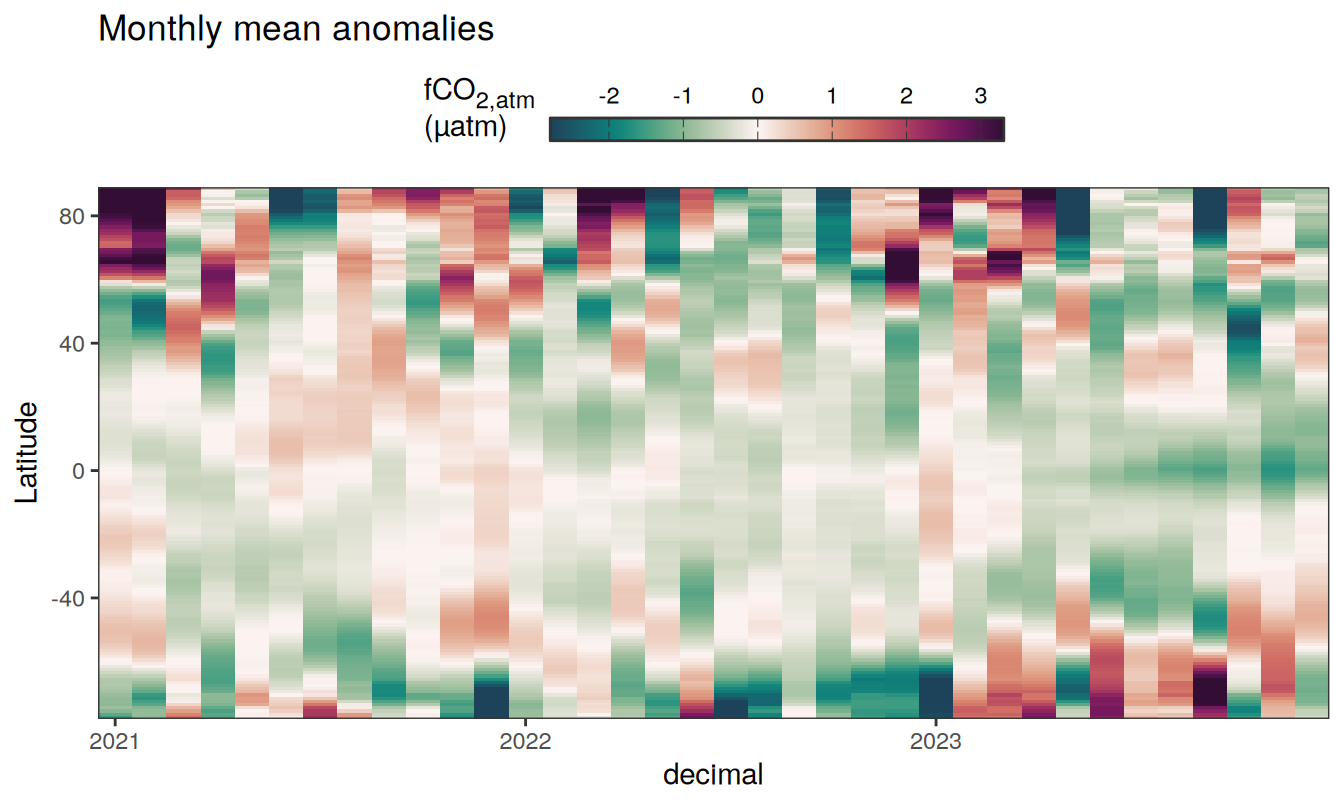
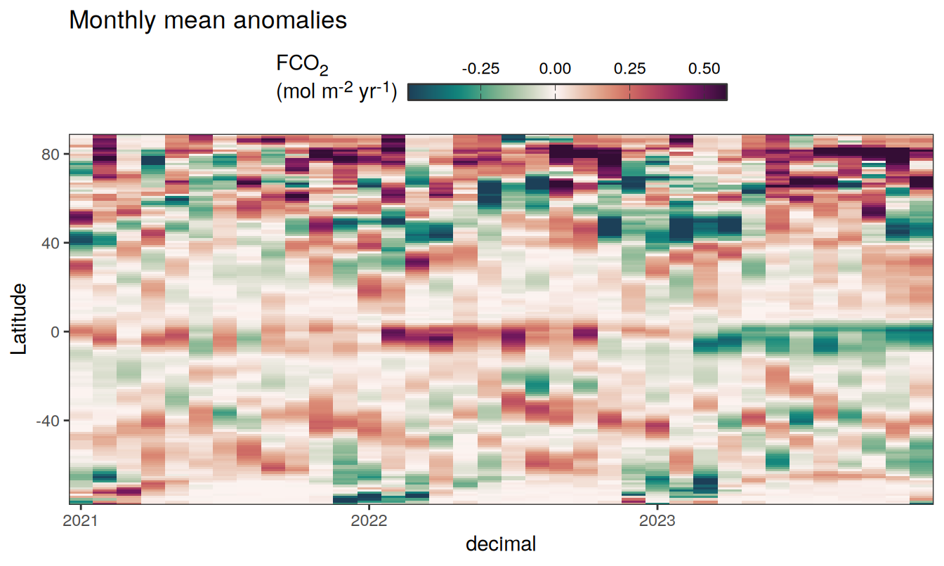
Three years prior 2023

pco2_product_hovmoeller_monthly_anomaly %>%
  filter(between(year, 2023-2, 2023)) %>%
  group_split(name) %>%
  # head(1) %>%
  map(
    ~ ggplot(data = .x,
             aes(decimal, lat, fill = resid)) +
      geom_raster() +
      scale_fill_gradientn(
        colours = cmocean("curl")(100),
        rescaler = ~ scales::rescale_mid(.x, mid = 0),
        name = labels_breaks(.x %>% distinct(name)),
        limits = c(quantile(.x$resid, .01), quantile(.x$resid, .99)),
        oob = squish
      ) +
      coord_cartesian(expand = 0) +
      labs(title = "Monthly mean anomalies",
           y = "Latitude") +
      guides(
        fill = guide_colorbar(
          barheight = unit(0.3, "cm"),
          barwidth = unit(6, "cm"),
          ticks = TRUE,
          ticks.colour = "grey20",
          frame.colour = "grey20",
          label.position = "top",
          direction = "horizontal"
        )
      ) +
      theme(legend.title = element_markdown(), legend.position = "top")
  )

pco2_product_hovmoeller_monthly_anomaly %>%
  write_csv(
    paste0(
      "../data/",
      "NIES-ML3_GCB",
      "_",
      "2023",
      "_hovmoeller_monthly_anomaly.csv"
    )
  )

rm(
  pco2_product_hovmoeller_annual,
  pco2_product_hovmoeller_monthly,
  pco2_product_hovmoeller_annual_anomaly,
  pco2_product_hovmoeller_monthly_anomaly
)

gc()

Regional means and integrals

The following plots show regionally averaged (or integrated) values of each variable as provided through the pCO2 product, as well as the anomalies from the prediction of a linear/quadratic fit.

Anomalies are first presented relative to the predicted annual mean of each year, hence preserving the seasonality. Furthermore, anomalies are presented relative to the predicted monthly mean values, such that the mean seasonality is removed.

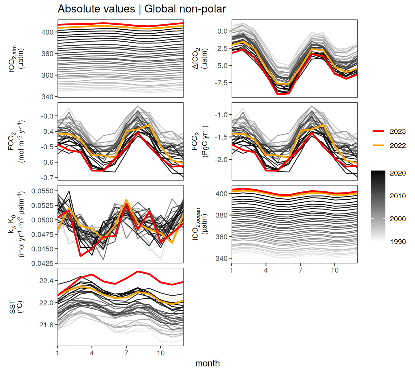
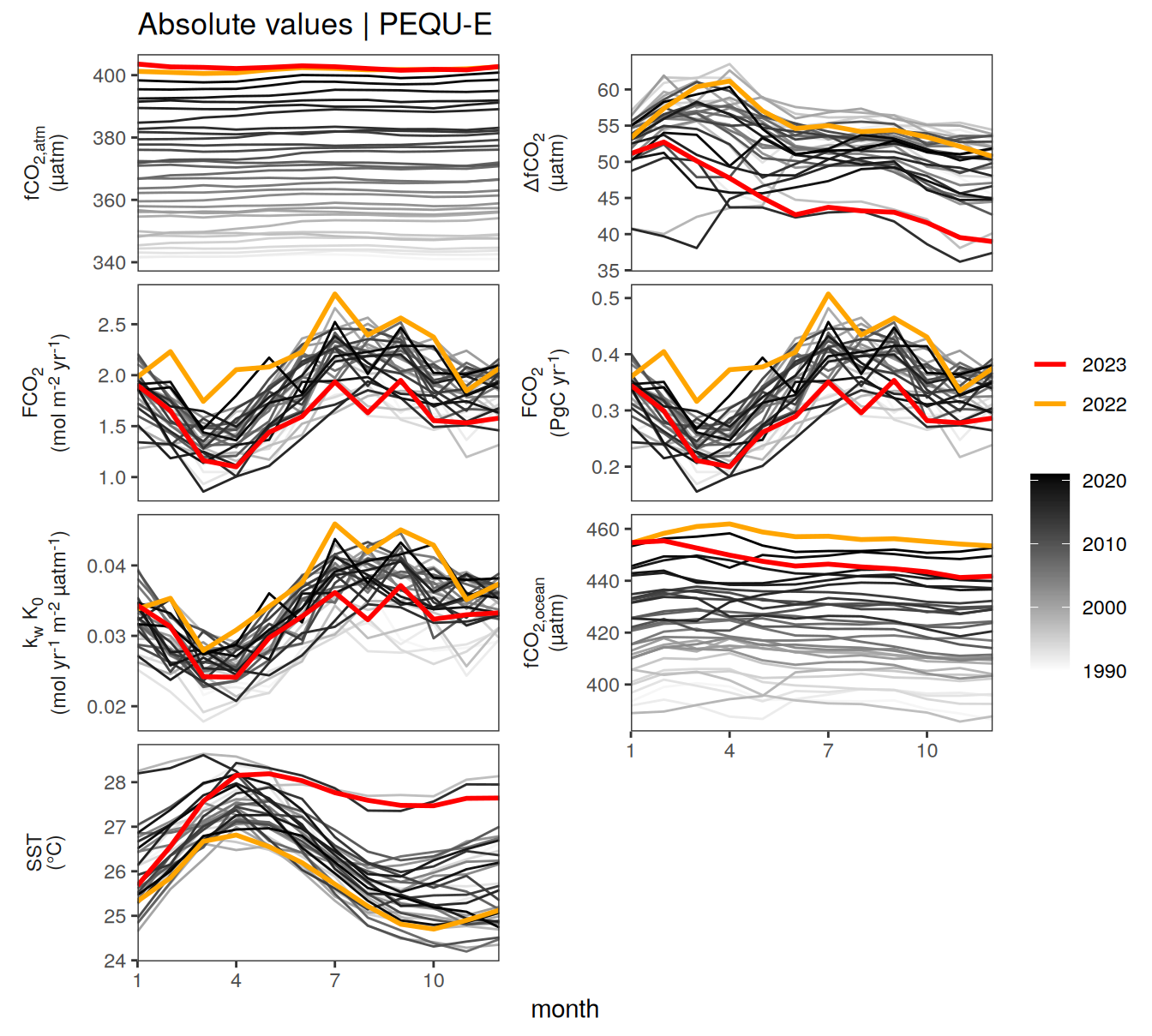
2023 absolute values

Global non-polar

fig.height <- pco2_product_biome_monthly %>% 
  distinct(name) %>% 
  nrow()

fig.height <- (fig.height + 2) * 0.1

pco2_product_biome_monthly %>%
  filter(biome %in% "Global non-polar") %>%
  ggplot(aes(month, value, group = as.factor(year))) +
  geom_path(data = . %>% filter(!between(year, 2023-1, 2023)),
            aes(col = year)) +
  scale_color_grayC() +
  new_scale_color() +
  geom_path(data = . %>% filter(between(year, 2023-1, 2023)),
            aes(col = as.factor(year)),
            linewidth = 1) +
  scale_color_manual(values = c("orange", "red"),
                     guide = guide_legend(reverse = TRUE,
                                          order = 1)) +
  scale_x_continuous(breaks = seq(1, 12, 3), expand = c(0, 0)) +
  labs(title = "Absolute values | Global non-polar") +
  facet_wrap(name ~ .,
             scales = "free_y",
             labeller = labeller(name = x_axis_labels),
             strip.position = "left",
             ncol = 2) +
  theme(
    strip.text.y.left = element_markdown(),
    strip.placement = "outside",
    strip.background.y = element_blank(),
    legend.title = element_blank(),
    axis.title.y = element_blank()
  )

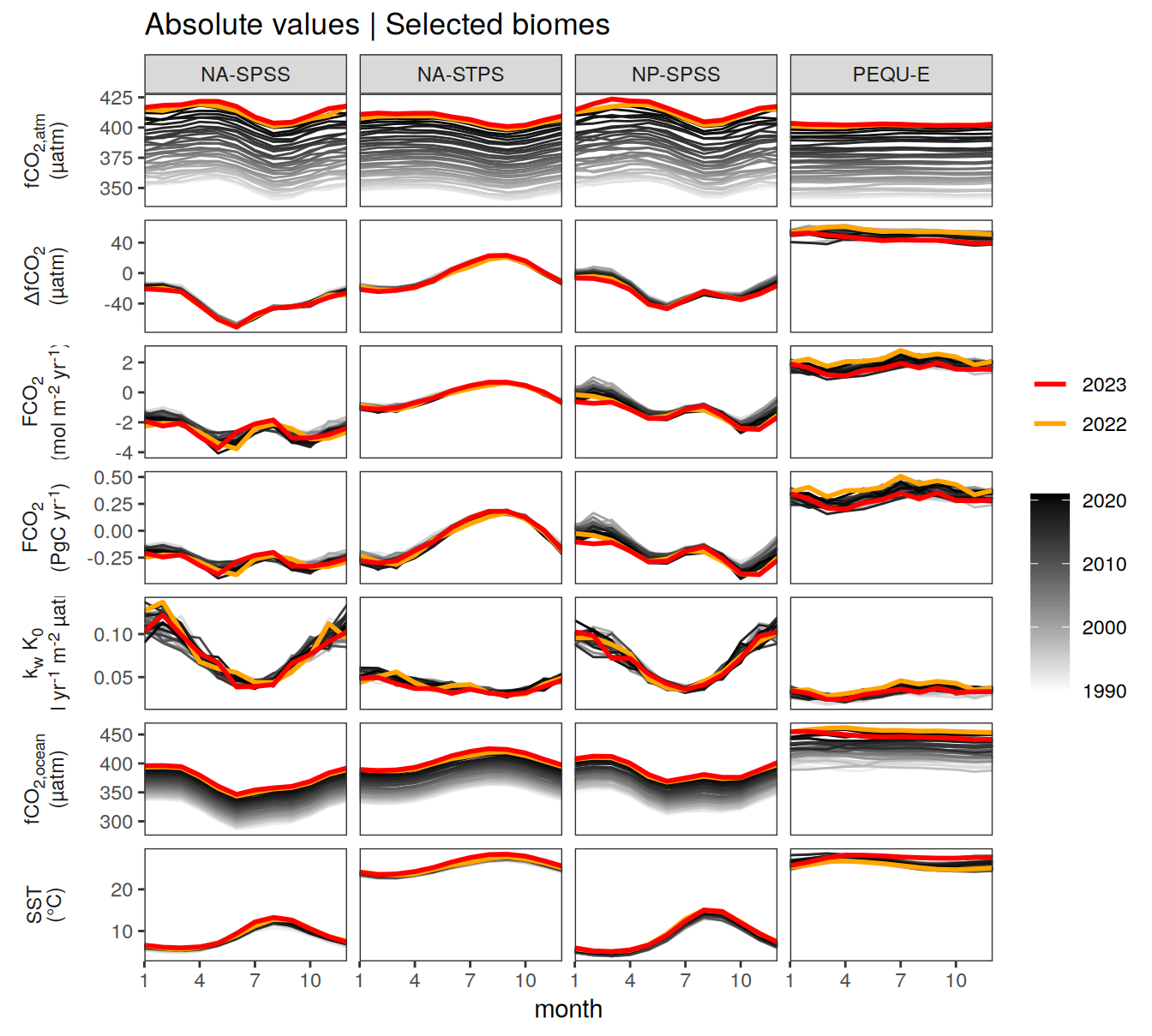
Key biomes

pco2_product_biome_monthly %>%
  filter(biome %in% key_biomes) %>%
  ggplot(aes(month, value, group = as.factor(year))) +
  geom_path(data = . %>% filter(!between(year, 2023-1, 2023)),
            aes(col = year)) +
  scale_color_grayC() +
  new_scale_color() +
  geom_path(data = . %>% filter(between(year, 2023-1, 2023)),
            aes(col = as.factor(year)),
            linewidth = 1) +
  scale_color_manual(values = c("orange", "red"),
                     guide = guide_legend(reverse = TRUE,
                                          order = 1)) +
  scale_x_continuous(breaks = seq(1, 12, 3), expand = c(0, 0)) +
  labs(title = "Absolute values | Selected biomes") +
  facet_grid(name ~ biome,
             scales = "free_y",
             labeller = labeller(name = x_axis_labels),
             switch = "y") +
  theme(
    strip.text.y.left = element_markdown(),
    strip.placement = "outside",
    strip.background.y = element_blank(),
    legend.title = element_blank(),
    axis.title.y = element_blank()
  )

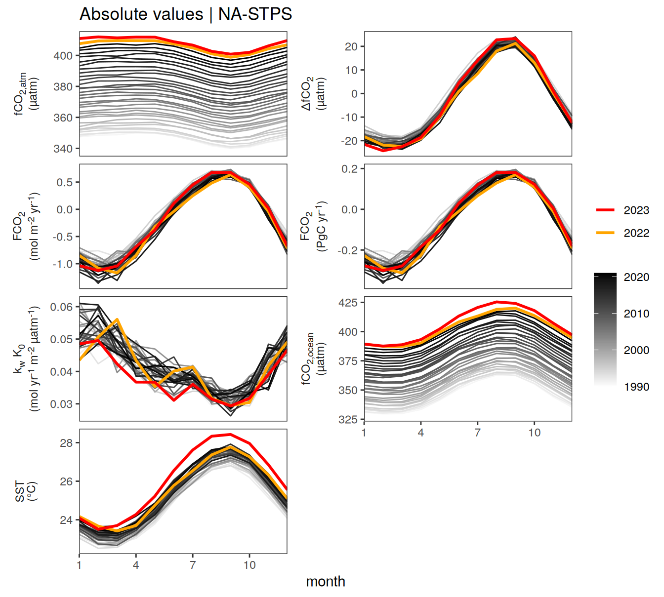
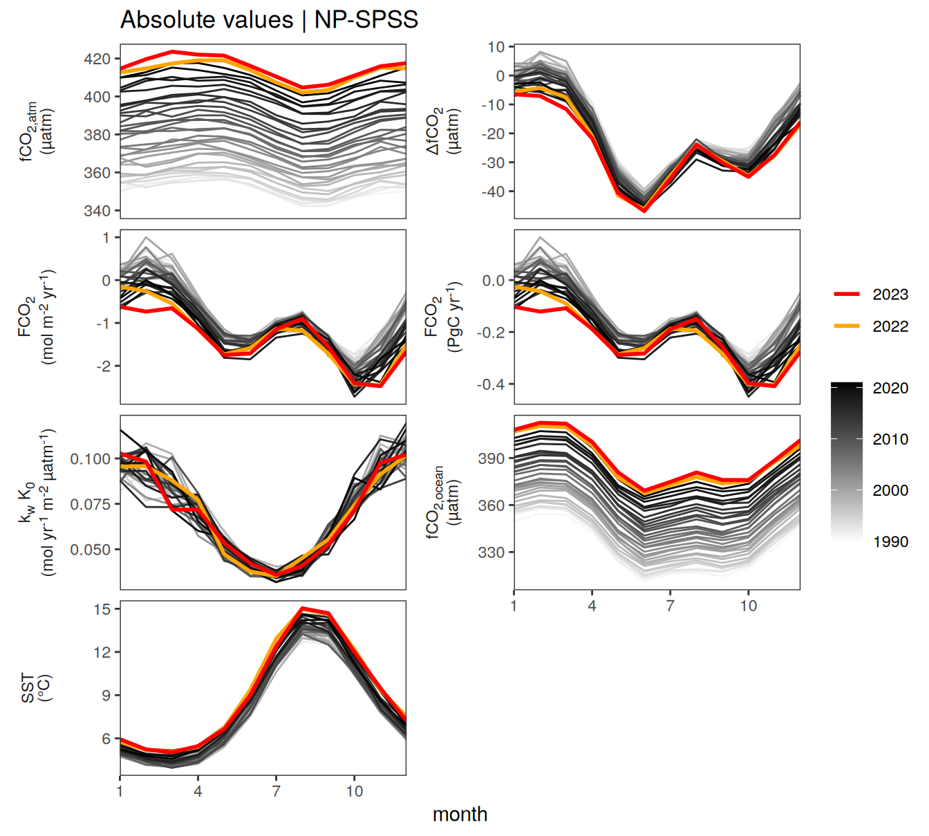
pco2_product_biome_monthly %>%
  filter(biome %in% key_biomes) %>%
  group_split(biome) %>%
  # head(1) %>%
  map(
    ~ ggplot(data = .x,
             aes(month, value, group = as.factor(year))) +
      geom_path(data = . %>% filter(!between(year, 2023-1, 2023)),
                aes(col = year)) +
      scale_color_grayC() +
      new_scale_color() +
      geom_path(
        data = . %>% filter(between(year, 2023-1, 2023)),
        aes(col = as.factor(year)),
        linewidth = 1
      ) +
      scale_color_manual(
        values = c("orange", "red"),
        guide = guide_legend(reverse = TRUE,
                             order = 1)
      ) +
      scale_x_continuous(breaks = seq(1, 12, 3), expand = c(0, 0)) +
  labs(title = paste("Absolute values |", .x$biome)) +
  facet_wrap(name ~ .,
             scales = "free_y",
             labeller = labeller(name = x_axis_labels),
             strip.position = "left",
             ncol = 2) +
  theme(
    strip.text.y.left = element_markdown(),
    strip.placement = "outside",
    strip.background.y = element_blank(),
    legend.title = element_blank(),
    axis.title.y = element_blank()
  )
  )

2023 anomalies

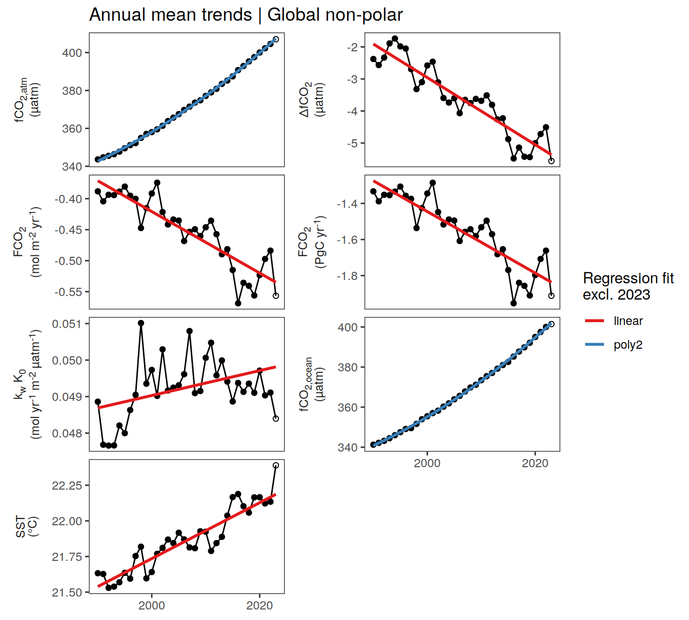
Annual mean trends

pco2_product_biome_annual %>% 
  filter(biome %in% "Global non-polar") %>%
  ggplot(aes(year, value)) +
  geom_path() +
  geom_point(data = . %>% filter(year != 2023)) +
  geom_point(data = . %>% filter(year == 2023),
             shape = 1) +
  geom_smooth(data = . %>% filter(year != 2023,
                                  !(name %in% name_quadratic_fit)),
              method = "lm",
              fullrange = TRUE,
              aes(col = "linear"),
              se = FALSE) +
  geom_smooth(data = . %>% filter(year != 2023,
                                  name %in% name_quadratic_fit),
              method = "lm",
              fullrange = TRUE,
              formula = y ~ poly(x,2),
              aes(col = "poly2"),
              se = FALSE) +
  scale_color_brewer(
    palette = "Set1",
    name = paste("Regression fit\nexcl.", 2023)) +
  scale_x_continuous(breaks = seq(1980, 2020, 20)) +
  labs(title = "Annual mean trends | Global non-polar") +
  facet_wrap(name ~ .,
             scales = "free_y",
             labeller = labeller(name = x_axis_labels),
             strip.position = "left",
             ncol = 2) +
  theme(
    strip.text.y.left = element_markdown(),
    strip.placement = "outside",
    strip.background.y = element_blank(),
    axis.title = element_blank()
  )

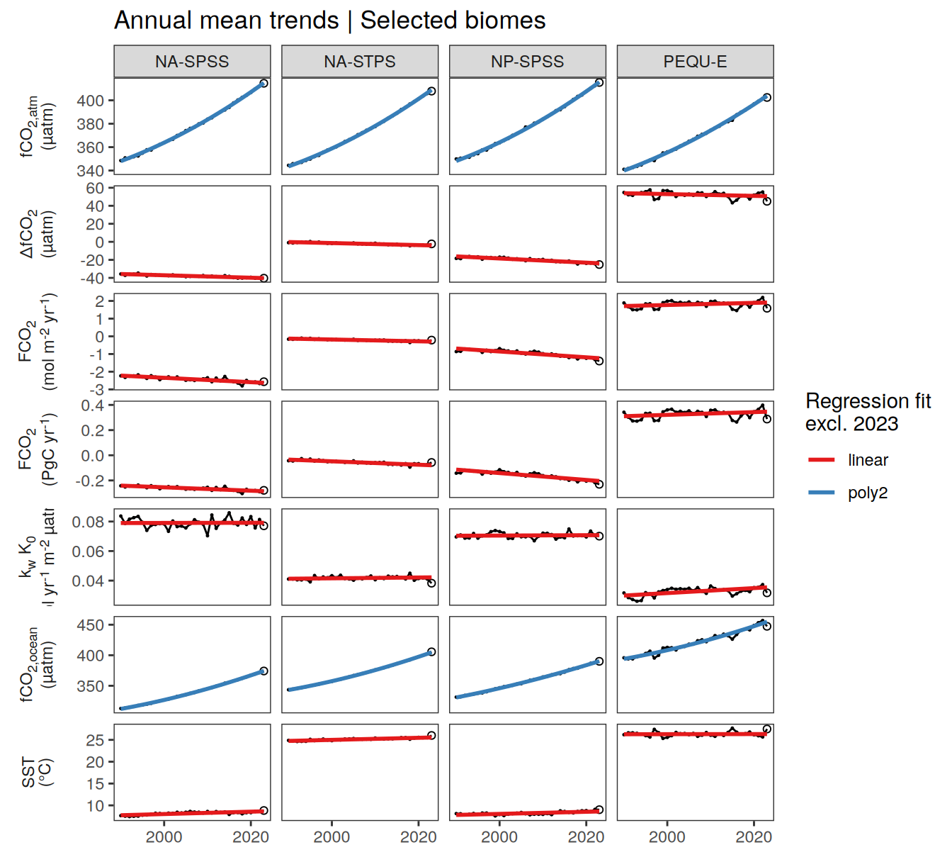
pco2_product_biome_annual %>% 
  filter(biome %in% key_biomes) %>%
  ggplot(aes(year, value)) +
  geom_path() +
  geom_point(data = . %>% filter(year != 2023),
             size = 0.2) +
  geom_point(data = . %>% filter(year == 2023),
             shape = 1) +
  geom_smooth(data = . %>% filter(year != 2023,
                                  !(name %in% name_quadratic_fit)),
              method = "lm",
              fullrange = TRUE,
              aes(col = "linear"),
              se = FALSE) +
  geom_smooth(data = . %>% filter(year != 2023,
                                  name %in% name_quadratic_fit),
              method = "lm",
              fullrange = TRUE,
              formula = y ~ poly(x,2),
              aes(col = "poly2"),
              se = FALSE) +
  scale_color_brewer(
    palette = "Set1",
    name = paste("Regression fit\nexcl.", 2023)) +
  scale_x_continuous(breaks = seq(1980, 2020, 20)) +
  labs(title = "Annual mean trends | Selected biomes") +
  facet_grid(name ~ biome,
             scales = "free_y",
             labeller = labeller(name = x_axis_labels),
             switch = "y") +
  theme(
    strip.text.y.left = element_markdown(),
    strip.placement = "outside",
    strip.background.y = element_blank(),
    axis.title = element_blank()
  )

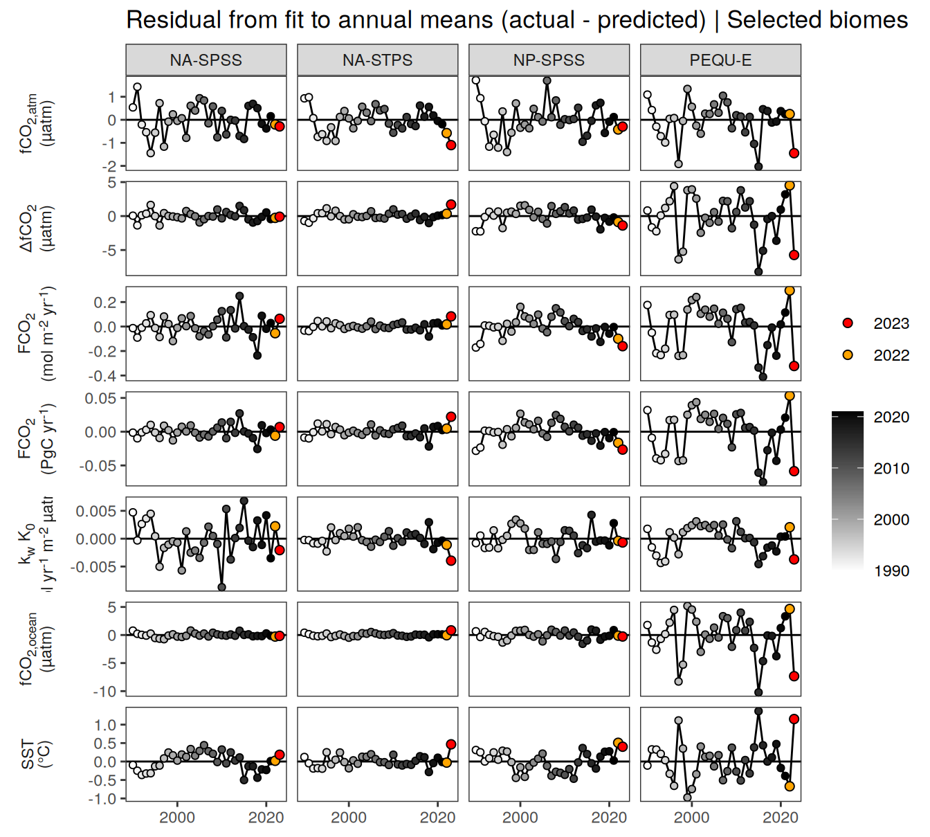
pco2_product_biome_annual_anomaly <-
  pco2_product_biome_annual %>%
  anomaly_determination(biome)
  

pco2_product_biome_annual_anomaly %>%
  filter(biome %in% "Global non-polar") %>%
  ggplot(aes(year, resid)) +
  geom_hline(yintercept = 0) +
  geom_path() +
  geom_point(data = . %>% filter(!between(year, 2023-1, 2023)),
             aes(fill = year),
             shape = 21) +
  scale_fill_grayC() +
  new_scale_fill() +
  geom_point(data = . %>% filter(between(year, 2023-1, 2023)),
             aes(fill = as.factor(year)),
             shape = 21, size = 2)  +
  scale_fill_manual(values = c("orange", "red"),
                     guide = guide_legend(reverse = TRUE,
                                          order = 1)) +
  scale_x_continuous(breaks = seq(1980, 2020, 20)) +
  labs(title = "Residual from fit to annual means (actual - predicted) | Global non-polar") +
  facet_wrap(name ~ .,
             scales = "free_y",
             labeller = labeller(name = x_axis_labels),
             strip.position = "left",
             ncol = 2) +
  theme(
    strip.text.y.left = element_markdown(),
    strip.placement = "outside",
    strip.background.y = element_blank(),
    axis.title = element_blank(),
    legend.title = element_blank()
  )

pco2_product_biome_annual_anomaly %>%
  filter(biome %in% key_biomes) %>%
  ggplot(aes(year, resid)) +
  geom_hline(yintercept = 0) +
  geom_path() +
  geom_point(data = . %>% filter(!between(year, 2023-1, 2023)),
             aes(fill = year),
             shape = 21) +
  scale_fill_grayC() +
  new_scale_fill() +
  geom_point(data = . %>% filter(between(year, 2023-1, 2023)),
             aes(fill = as.factor(year)),
             shape = 21, size = 2)  +
  scale_fill_manual(values = c("orange", "red"),
                     guide = guide_legend(reverse = TRUE,
                                          order = 1)) +
  scale_x_continuous(breaks = seq(1980, 2020, 20)) +
  labs(title = "Residual from fit to annual means (actual - predicted) | Selected biomes") +
  facet_grid(name ~ biome,
             scales = "free_y",
             labeller = labeller(name = x_axis_labels),
             switch = "y") +
  theme(
    strip.text.y.left = element_markdown(),
    strip.placement = "outside",
    strip.background.y = element_blank(),
    axis.title = element_blank(),
    legend.title = element_blank()
  )

pco2_product_biome_annual_anomaly %>%
  write_csv(
    paste0(
      "../data/",
      "NIES-ML3_GCB",
      "_",
      "2023",
      "_biome_annual_anomaly.csv"
    )
  )

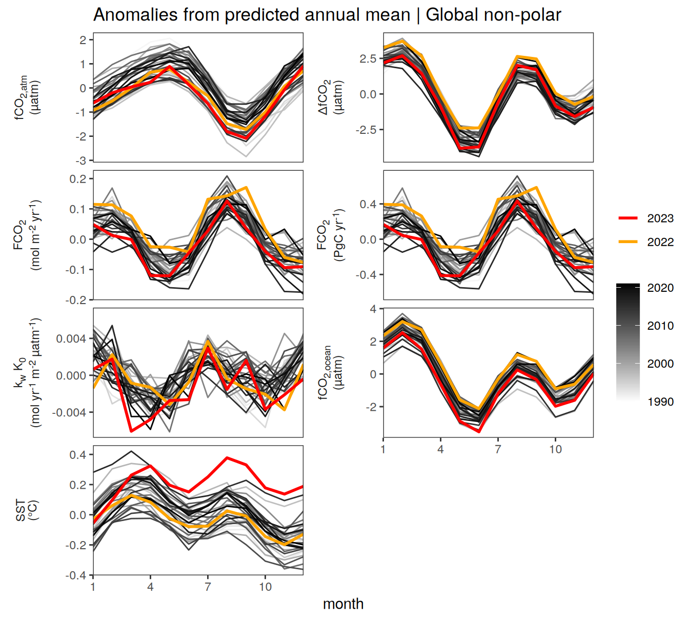
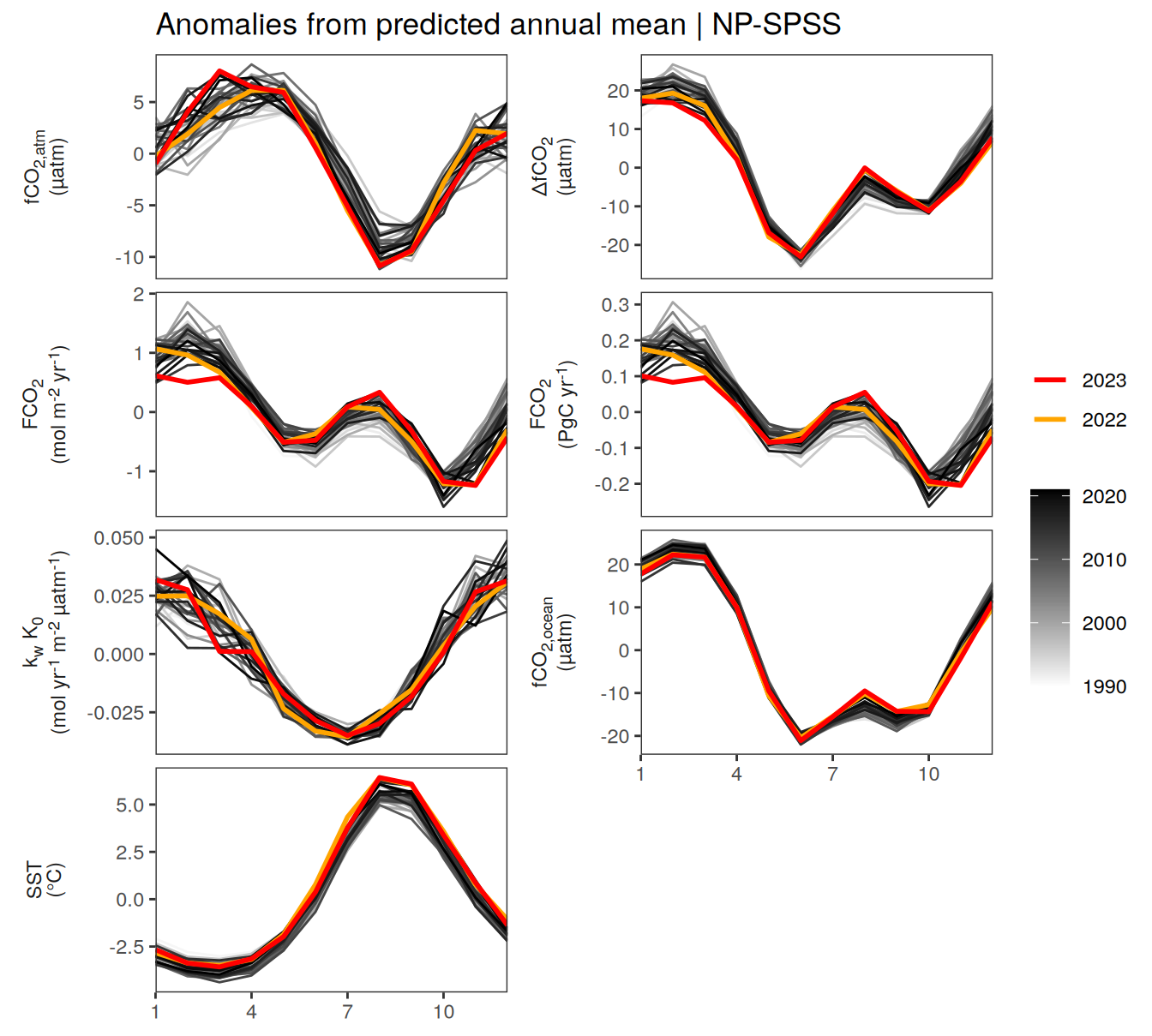
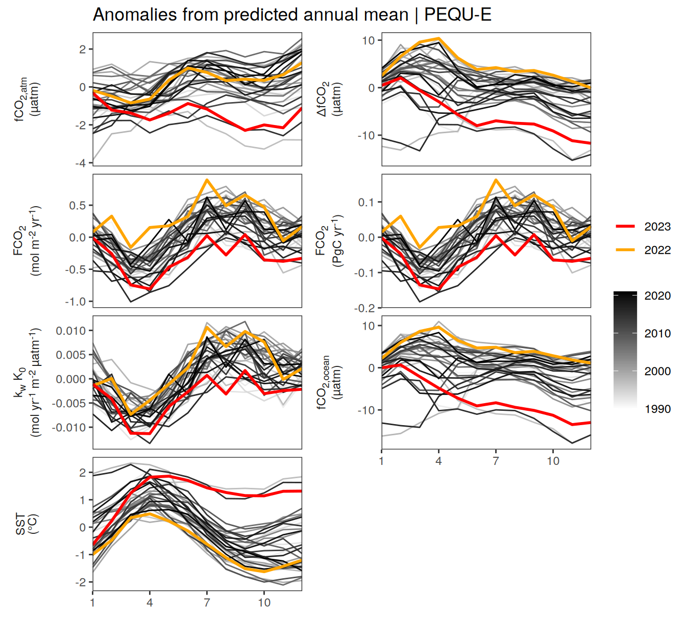
pco2_product_biome_annual_detrended <-
  full_join(pco2_product_biome_monthly,
            pco2_product_biome_annual_anomaly %>% select(-c(value, resid))) %>%
  mutate(resid = value - fit)

pco2_product_biome_annual_detrended %>% 
  filter(biome %in% "Global non-polar") %>%
  ggplot(aes(month, resid, group = as.factor(year))) +
  geom_path(data = . %>% filter(!between(year, 2023-1, 2023)),
            aes(col = year)) +
  scale_color_grayC() +
  new_scale_color() +
  geom_path(data = . %>% filter(between(year, 2023-1, 2023)),
            aes(col = as.factor(year)),
            linewidth = 1) +
  scale_color_manual(values = c("orange", "red"),
                     guide = guide_legend(reverse = TRUE,
                                          order = 1)) +
  scale_x_continuous(breaks = seq(1, 12, 3), expand = c(0, 0)) +
  labs(title = "Anomalies from predicted annual mean | Global non-polar") +
  facet_wrap(name ~ .,
             scales = "free_y",
             labeller = labeller(name = x_axis_labels),
             strip.position = "left",
             ncol = 2) +
  theme(
    strip.text.y.left = element_markdown(),
    strip.placement = "outside",
    strip.background.y = element_blank(),
    axis.title.y = element_blank(),
    legend.title = element_blank()
  )

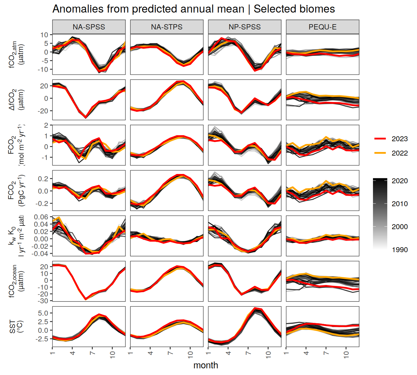
pco2_product_biome_annual_detrended %>% 
  filter(biome %in% key_biomes) %>%
  ggplot(aes(month, resid, group = as.factor(year))) +
  geom_path(data = . %>% filter(!between(year, 2023-1, 2023)),
            aes(col = year)) +
  scale_color_grayC() +
  new_scale_color() +
  geom_path(data = . %>% filter(between(year, 2023-1, 2023)),
            aes(col = as.factor(year)),
            linewidth = 1) +
  scale_color_manual(values = c("orange", "red"),
                     guide = guide_legend(reverse = TRUE,
                                          order = 1)) +
  scale_x_continuous(breaks = seq(1, 12, 3), expand = c(0, 0)) +
  labs(title = "Anomalies from predicted annual mean | Selected biomes") +
  facet_grid(name ~ biome,
             scales = "free_y",
             labeller = labeller(name = x_axis_labels),
             switch = "y") +
  theme(
    strip.text.y.left = element_markdown(),
    strip.placement = "outside",
    strip.background.y = element_blank(),
    axis.title.y = element_blank(),
    legend.title = element_blank(),
        axis.text.x = element_text(angle = 90, vjust = 0.5, hjust=1)
  )

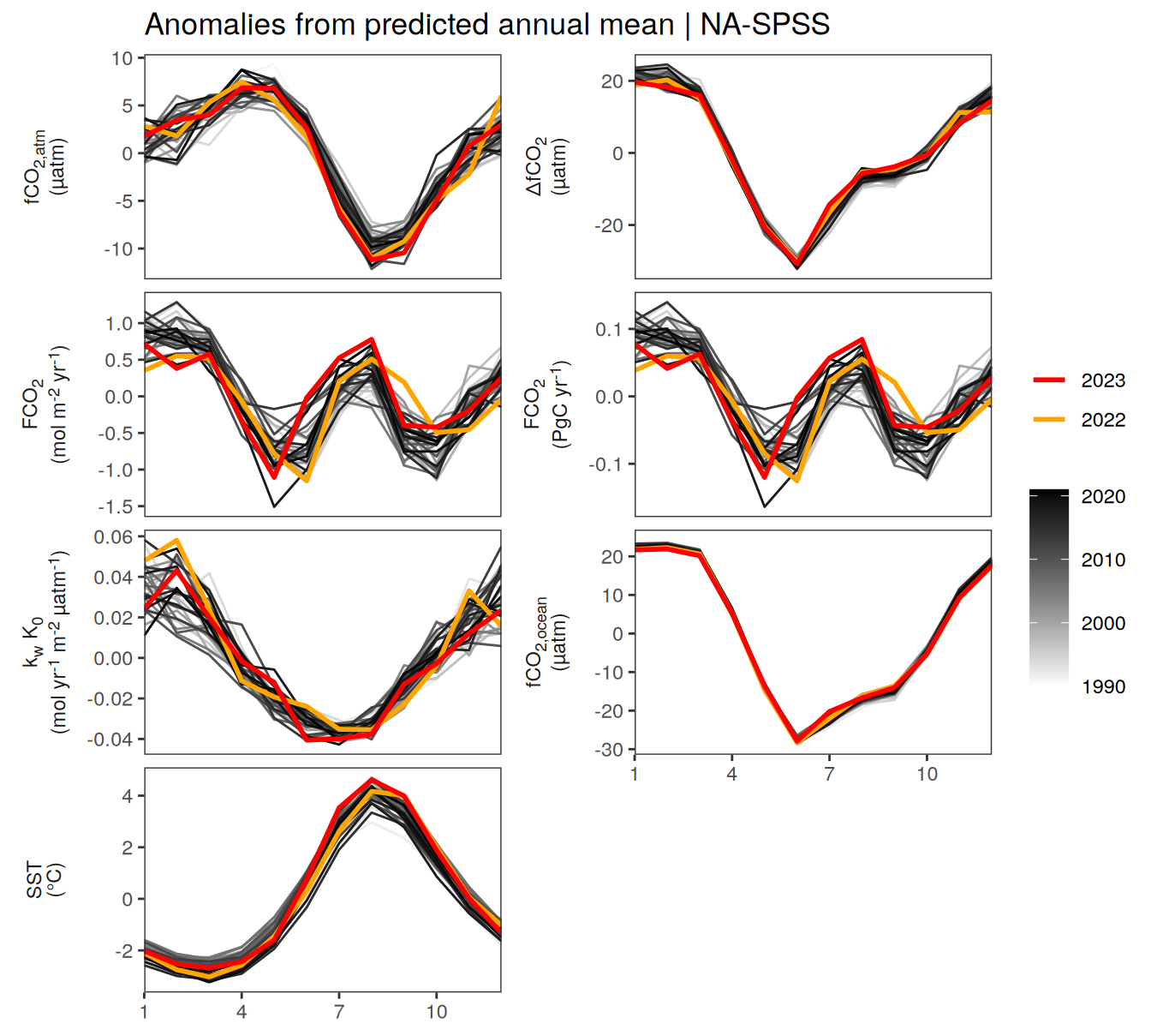
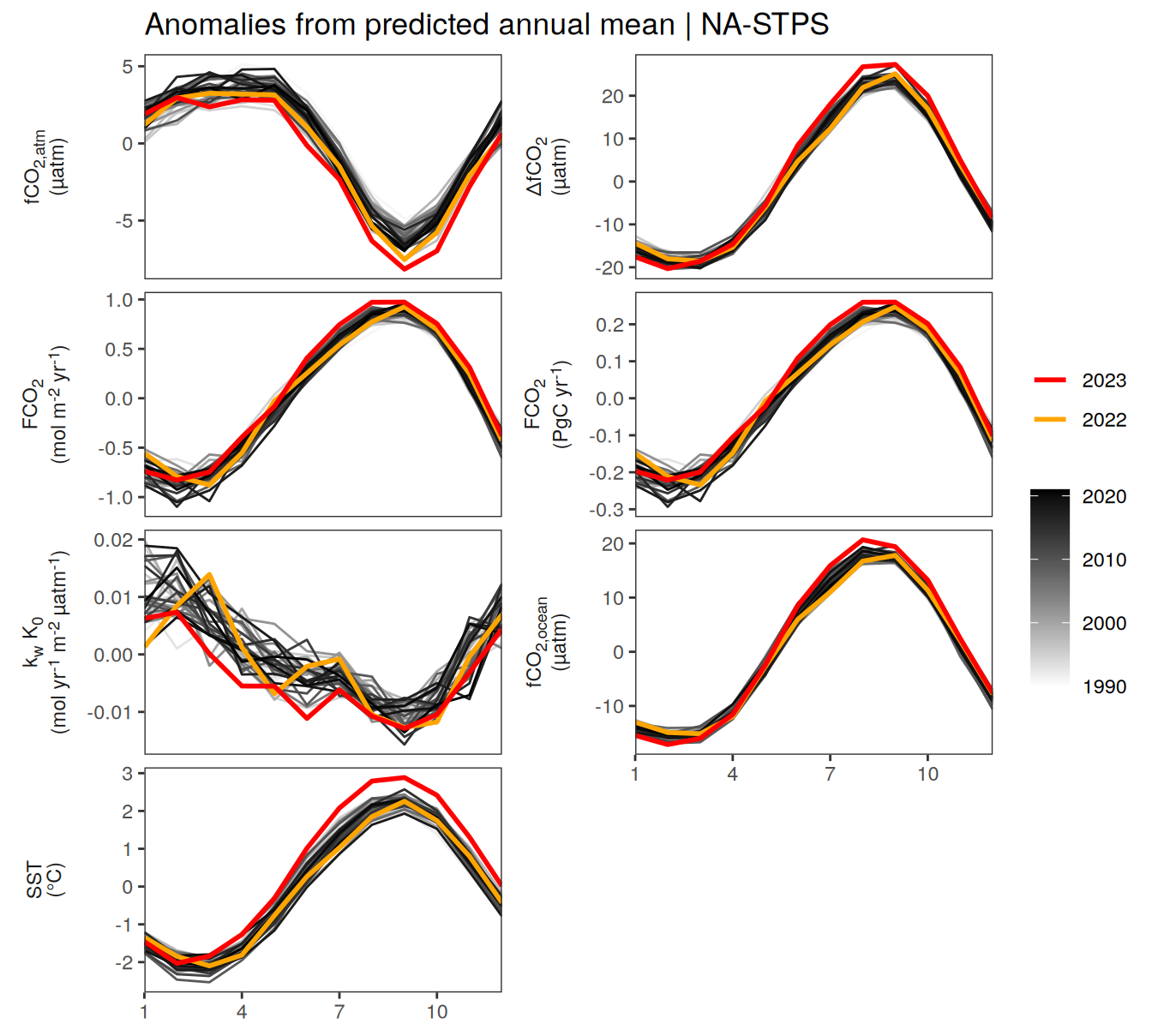
pco2_product_biome_annual_detrended %>%
  filter(biome %in% key_biomes) %>%
  group_split(biome) %>%
  # head(1) %>%
  map(
    ~ ggplot(data = .x,
             aes(month, resid, group = as.factor(year))) +
      geom_path(data = . %>% filter(!between(year, 2023-1, 2023)),
                aes(col = year)) +
      scale_color_grayC() +
      new_scale_color() +
      geom_path(
        data = . %>% filter(between(year, 2023-1, 2023)),
        aes(col = as.factor(year)),
        linewidth = 1
      ) +
      scale_color_manual(
        values = c("orange", "red"),
        guide = guide_legend(reverse = TRUE,
                             order = 1)
      ) +
      scale_x_continuous(breaks = seq(1, 12, 3), expand = c(0, 0)) +
      labs(title = paste("Anomalies from predicted annual mean |", .x$biome)) +
      facet_wrap(
        name ~ .,
        scales = "free_y",
        labeller = labeller(name = x_axis_labels),
        strip.position = "left",
        ncol = 2
      ) +
      theme(
        strip.text.y.left = element_markdown(),
        strip.placement = "outside",
        strip.background.y = element_blank(),
        axis.title = element_blank(),
        legend.title = element_blank()
      )
  )

pco2_product_biome_annual_detrended %>%
  write_csv(
    paste0(
      "../data/",
      "NIES-ML3_GCB",
      "_",
      "2023",
      "_biome_annual_detrended.csv"
    )
  )

Monthly mean trends

# pco2_product_biome_monthly %>% 
#   filter(biome %in% "Global non-polar") %>%
#   mutate(month = as.factor(month)) %>% 
#   ggplot(aes(year, value, col = month)) +
#   # geom_point() +
#   geom_smooth(data = . %>% filter(year != 2023,
#                                   !(name %in% name_quadratic_fit)),
#               method = "lm",
#               se = FALSE,
#               fullrange = TRUE) +
#   geom_smooth(
#     data = . %>% filter(year != 2023,
#                         name %in% name_quadratic_fit),
#     method = "lm",
#     fullrange = TRUE,
#     formula = y ~ x + I(x ^ 2),
#     se = FALSE
#   ) +
#   scale_color_scico_d(palette = "romaO", 
#     name = paste("Regression fit\nexcl.", 2023)) +
#   scale_x_continuous(breaks = seq(1980, 2020, 20)) +
#   labs(title = "Monthly mean trends | Global non-polar") +
#   facet_wrap(name ~ .,
#              scales = "free_y",
#              labeller = labeller(name = x_axis_labels),
#              strip.position = "left",
#              ncol = 2) +
#   theme(
#     strip.text.y.left = element_markdown(),
#     strip.placement = "outside",
#     strip.background.y = element_blank(),
#     axis.title = element_blank()
#   )
# 
# pco2_product_biome_monthly %>% 
#   filter(biome %in% key_biomes) %>%
#   mutate(month = as.factor(month)) %>% 
#   ggplot(aes(year, value, col = month)) +
#   # geom_point() +
#   geom_smooth(data = . %>% filter(year != 2023,
#                                   !(name %in% name_quadratic_fit)),
#               method = "lm",
#               fullrange = TRUE,
#               se = FALSE) +
#   geom_smooth(
#     data = . %>% filter(year != 2023,
#                         name %in% name_quadratic_fit),
#     method = "lm",
#     fullrange = TRUE,
#     formula = y ~ x + I(x ^ 2),
#     se = FALSE
#   ) +
#   scale_color_scico_d(palette = "romaO",
#     name = paste("Regression fit\nexcl.", 2023)) +
#   scale_x_continuous(breaks = seq(1980, 2020, 20)) +
#   labs(title = "Monthly mean trends | Selected biomes") +
#   facet_grid(name ~ biome,
#              scales = "free_y",
#              labeller = labeller(name = x_axis_labels),
#              switch = "y") +
#   theme(
#     strip.text.y.left = element_markdown(),
#     strip.placement = "outside",
#     strip.background.y = element_blank(),
#     axis.title = element_blank()
#   )

pco2_product_biome_monthly_anomaly <-
  pco2_product_biome_monthly %>%
  anomaly_determination(biome, month)


# pco2_product_biome_monthly_anomaly %>%
#   filter(biome %in% "Global non-polar") %>%
#   group_split(month) %>%
#   head(1) %>%
#   map(
#     ~ ggplot(data = .x,
#              aes(year, resid)) +
#       geom_hline(yintercept = 0) +
#       geom_path() +
#       geom_point(
#         data = . %>% filter(!between(year, 2023-1, 2023)),
#         aes(fill = year),
#         shape = 21
#       ) +
#       scale_fill_grayC() +
#       new_scale_fill() +
#       geom_point(
#         data = . %>% filter(between(year, 2023-1, 2023)),
#         aes(fill = as.factor(year)),
#         shape = 21,
#         size = 2
#       )  +
#       scale_fill_manual(
#         values = c("orange", "red"),
#         guide = guide_legend(reverse = TRUE,
#                              order = 1)
#       ) +
#       scale_x_continuous(breaks = seq(1980, 2020, 20)) +
#       labs(title = "Residual from fit to monthly means (actual - predicted) | Global non-polar",
#            subtitle = paste("Month:", .x$month)) +
#       facet_wrap(
#         name ~ .,
#         scales = "free_y",
#         labeller = labeller(name = x_axis_labels),
#         strip.position = "left",
#         ncol = 2
#       ) +
#       theme(
#         strip.text.y.left = element_markdown(),
#         strip.placement = "outside",
#         strip.background.y = element_blank(),
#         axis.title = element_blank(),
#         legend.title = element_blank()
#       )
#   )
# 
# pco2_product_biome_monthly_anomaly %>%
#   filter(biome %in% key_biomes) %>%
#   group_split(month) %>%
#   head(1) %>%
#   map(
#     ~ ggplot(data = .x,
#              aes(year, resid)) +
#       geom_hline(yintercept = 0) +
#       geom_path() +
#       geom_point(
#         data = . %>% filter(!between(year, 2023-1, 2023)),
#         aes(fill = year),
#         shape = 21
#       ) +
#       scale_fill_grayC() +
#       new_scale_fill() +
#       geom_point(
#         data = . %>% filter(between(year, 2023-1, 2023)),
#         aes(fill = as.factor(year)),
#         shape = 21,
#         size = 2
#       )  +
#       scale_fill_manual(
#         values = c("orange", "red"),
#         guide = guide_legend(reverse = TRUE,
#                              order = 1)
#       ) +
#       scale_x_continuous(breaks = seq(1980, 2020, 20)) +
#       labs(title = "Residual from fit to monthly means (actual - predicted) | Selected biomes",
#            subtitle = paste("Month:", .x$month)) +
#       facet_grid(
#         name ~ biome,
#         scales = "free_y",
#         labeller = labeller(name = x_axis_labels),
#         switch = "y"
#       ) +
#       theme(
#         strip.text.y.left = element_markdown(),
#         strip.placement = "outside",
#         strip.background.y = element_blank(),
#         axis.title = element_blank(),
#         legend.title = element_blank()
#       )
#   )

pco2_product_biome_monthly_anomaly %>%
  write_csv(
    paste0(
      "../data/",
      "NIES-ML3_GCB",
      "_",
      "2023",
      "_biome_monthly_anomaly.csv"
    )
  )

Global non-polar

pco2_product_biome_monthly_detrended <-
  full_join(pco2_product_biome_monthly,
            pco2_product_biome_monthly_anomaly %>% select(-c(value, resid))) %>%
  mutate(resid = value - fit)

pco2_product_biome_monthly_detrended %>% 
  filter(biome %in% "Global non-polar") %>%
  ggplot(aes(month, resid, group = as.factor(year))) +
  geom_path(data = . %>% filter(!between(year, 2023-1, 2023)),
            aes(col = year)) +
  scale_color_grayC() +
  new_scale_color() +
  geom_path(data = . %>% filter(between(year, 2023-1, 2023)),
            aes(col = as.factor(year)),
            linewidth = 1) +
  scale_color_manual(values = c("orange", "red"),
                     guide = guide_legend(reverse = TRUE,
                                          order = 1)) +
  scale_x_continuous(breaks = seq(1, 12, 3), expand = c(0, 0)) +
  labs(title = "Anomalies from predicted monthly mean | Global non-polar") +
  facet_wrap(
    name ~ .,
    scales = "free_y",
    labeller = labeller(name = x_axis_labels),
    strip.position = "left",
    ncol = 2
  ) +
  theme(
    strip.text.y.left = element_markdown(),
    strip.placement = "outside",
    strip.background.y = element_blank(),
    axis.title.y = element_blank(),
    legend.title = element_blank()
  )

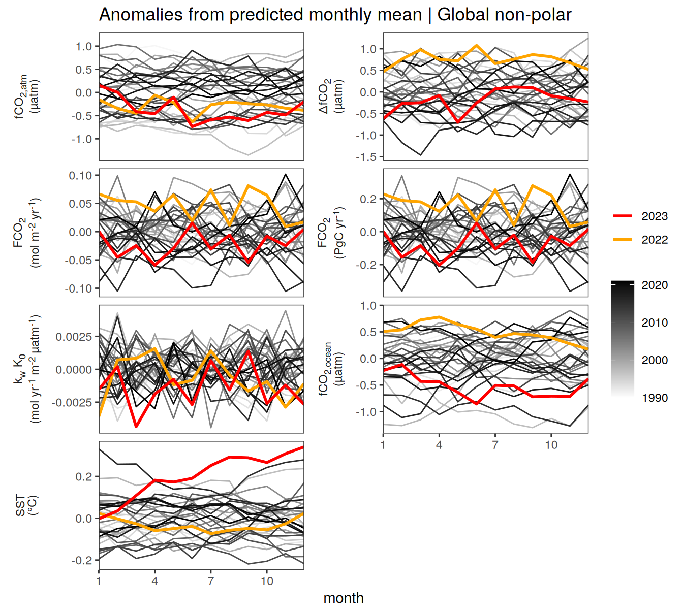
pco2_product_biome_monthly_detrended %>% 
  filter(biome %in% key_biomes) %>%
  ggplot(aes(month, resid, group = as.factor(year))) +
  geom_path(data = . %>% filter(!between(year, 2023-1, 2023)),
            aes(col = year)) +
  scale_color_grayC() +
  new_scale_color() +
  geom_path(data = . %>% filter(between(year, 2023-1, 2023)),
            aes(col = as.factor(year)),
            linewidth = 1) +
  scale_color_manual(values = c("orange", "red"),
                     guide = guide_legend(reverse = TRUE,
                                          order = 1)) +
  scale_x_continuous(breaks = seq(1, 12, 3), expand = c(0, 0)) +
  labs(title = "Anomalies from predicted monthly mean | Selected biomes") +
  facet_grid(
    name ~ biome,
    scales = "free_y",
    labeller = labeller(name = x_axis_labels),
    switch = "y"
  ) +
  theme(
    strip.text.y.left = element_markdown(),
    strip.placement = "outside",
    strip.background.y = element_blank(),
    axis.title.y = element_blank(),
    legend.title = element_blank()
  )

Key biomes

pco2_product_biome_monthly_detrended %>% 
  filter(biome %in% key_biomes) %>%
  ggplot(aes(month, resid, group = as.factor(year))) +
  geom_path(data = . %>% filter(!between(year, 2023-1, 2023)),
            aes(col = year)) +
  scale_color_grayC() +
  new_scale_color() +
  geom_path(data = . %>% filter(between(year, 2023-1, 2023)),
            aes(col = as.factor(year)),
            linewidth = 1) +
  scale_color_manual(values = c("orange", "red"),
                     guide = guide_legend(reverse = TRUE,
                                          order = 1)) +
  scale_x_continuous(breaks = seq(1, 12, 3), expand = c(0, 0)) +
  labs(title = "Anomalies from predicted monthly mean | Selected biomes") +
  facet_grid(
    name ~ biome,
    scales = "free_y",
    labeller = labeller(name = x_axis_labels),
    switch = "y"
  ) +
  theme(
    strip.text.y.left = element_markdown(),
    strip.placement = "outside",
    strip.background.y = element_blank(),
    axis.title.y = element_blank(),
    legend.title = element_blank()
  )

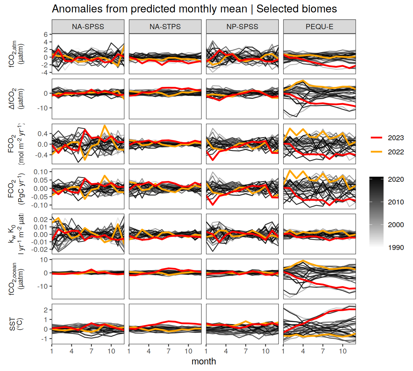
pco2_product_biome_monthly_detrended %>%
  filter(biome %in% key_biomes) %>%
  group_split(biome) %>%
  # head(1) %>%
  map(
    ~ ggplot(data = .x,
             aes(month, resid, group = as.factor(year))) +
      geom_path(data = . %>% filter(!between(year, 2023-1, 2023)),
                aes(col = year)) +
      scale_color_grayC() +
      new_scale_color() +
      geom_path(
        data = . %>% filter(between(year, 2023-1, 2023)),
        aes(col = as.factor(year)),
        linewidth = 1
      ) +
      scale_color_manual(
        values = c("orange", "red"),
        guide = guide_legend(reverse = TRUE,
                             order = 1)
      ) +
      scale_x_continuous(breaks = seq(1, 12, 3), expand = c(0, 0)) +
      labs(title = paste("Anomalies from predicted monthly mean |", .x$biome)) +
      facet_wrap(
        name ~ .,
        scales = "free_y",
        labeller = labeller(name = x_axis_labels),
        strip.position = "left",
        ncol = 2
      ) +
      theme(
        strip.text.y.left = element_markdown(),
        strip.placement = "outside",
        strip.background.y = element_blank(),
        axis.title.y = element_blank(),
        legend.title = element_blank()
      )
  )

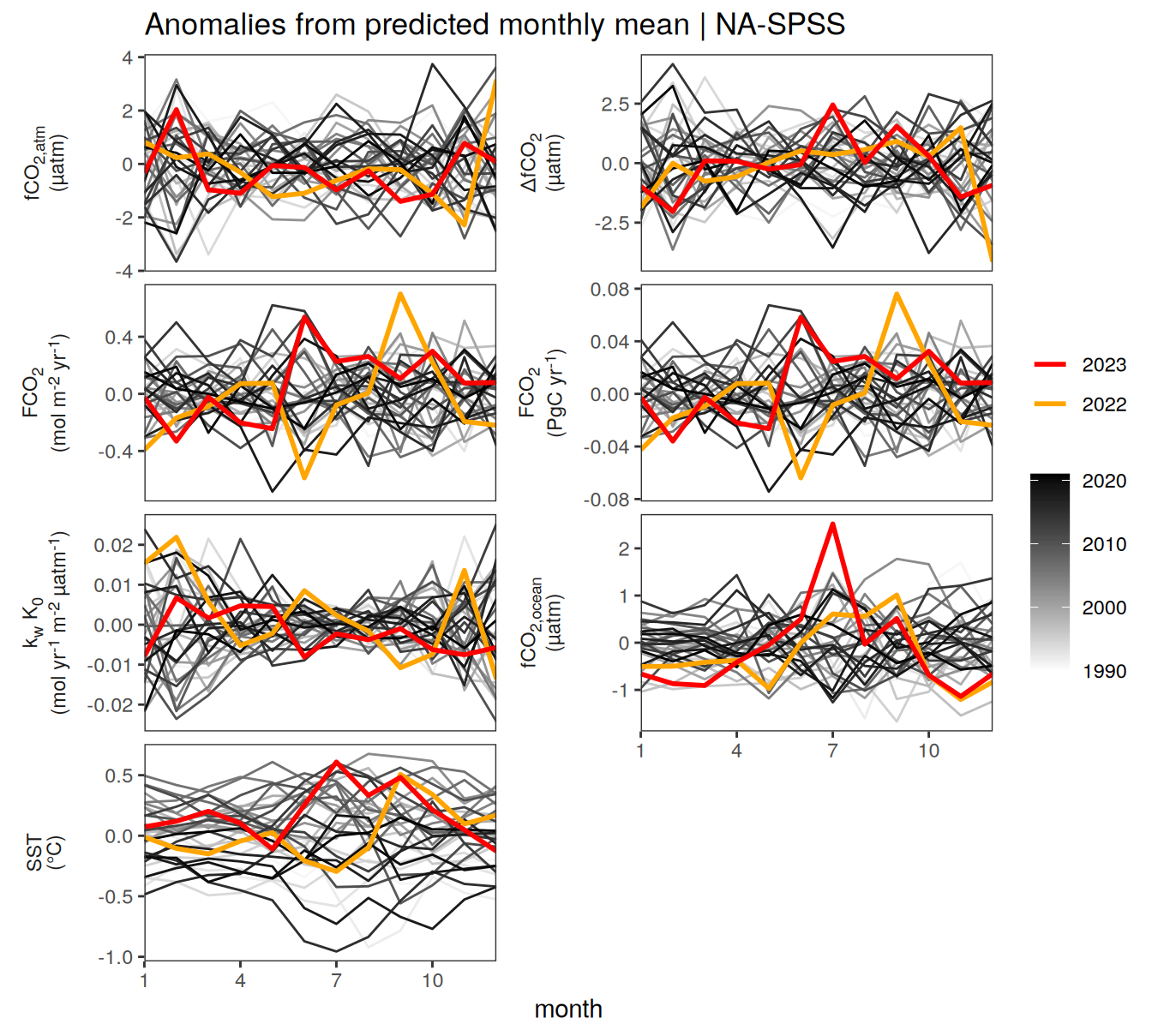
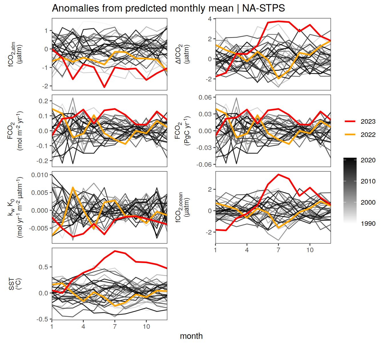
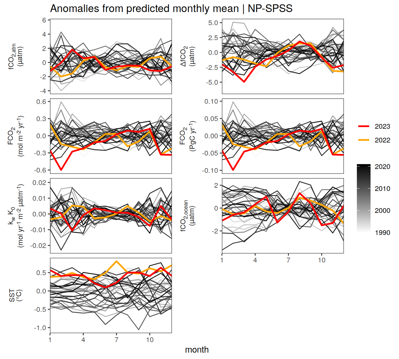
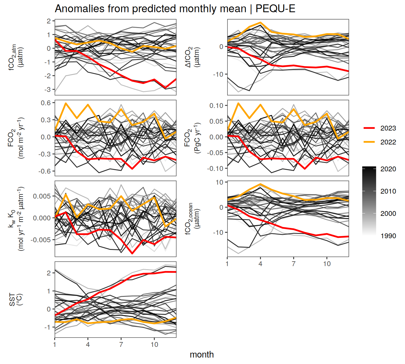
pco2_product_biome_monthly_detrended %>%
  write_csv(
    paste0(
      "../data/",
      "NIES-ML3_GCB",
      "_",
      "2023",
      "_biome_monthly_detrended.csv"
    )
  )

2023 anomaly correlation

The following plots aim to unravel the correlation between regionally integrated monthly flux anomalies and the corresponding anomalies of the means/integrals of each other variable.

Anomalies are first presented are first presented in absolute units. Due to the different flux magnitudes, we need to plot integrated fluxes separately for each region. Secondly, we normalize the monthly anomalies to the spread (expressed as standard deviation) of the residuals from the fit.

Annual anomalies

Absolute

pco2_product_biome_annual_anomaly %>%
  filter(biome == "Global non-polar") %>%
  select(-c(value, fit)) %>% 
  pivot_wider(values_from = resid) %>% 
  pivot_longer(-c(year, biome, fgco2_int))  %>%
  ggplot(aes(value, fgco2_int)) +
  geom_hline(yintercept = 0) +
  geom_point(data = . %>% filter(!between(year, 2023-1, 2023)),
             aes(fill = year),
             shape = 21) +
  geom_smooth(
    data = . %>% filter(!between(year, 2023-1, 2023)),
    method = "lm",
    se = FALSE,
    fullrange = TRUE,
    aes(col = paste("Regression fit\nexcl.", 2023))
  ) +
  scale_color_grey() +
  scale_fill_grayC()+
  new_scale_fill() +
  geom_point(data = . %>% filter(between(year, 2023-1, 2023)),
             aes(fill = as.factor(year)),
             shape = 21, size = 2)  +
  scale_fill_manual(values = c("orange", "red"),
                     guide = guide_legend(reverse = TRUE,
                                          order = 1)) +
  labs(title = "Global non-polar integrated fluxes",
       y = labels_breaks("fgco2_int")$i_legend_title) +
  facet_wrap(
    ~ name,
    scales = "free_x",
    labeller = labeller(name = x_axis_labels),
    strip.position = "bottom",
    ncol = 2
  ) +
  theme(
    strip.text.x.bottom = element_markdown(),
    strip.placement = "outside",
    strip.background.x = element_blank(),
    axis.title.y = element_markdown(),
    axis.title.x = element_blank(),
    legend.title = element_blank()
  )

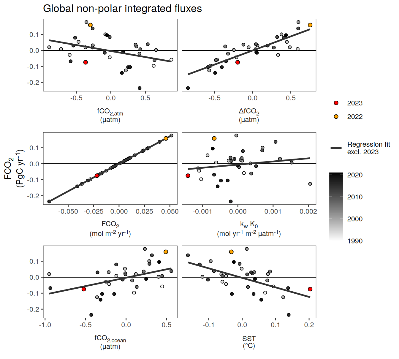
Monthly anomalies

Absolute

pco2_product_biome_monthly_detrended_anomaly <-
  pco2_product_biome_monthly_detrended %>%
  select(year, month, biome, name, resid) %>%
  pivot_wider(names_from = name,
              values_from = resid)


pco2_product_biome_monthly_detrended_anomaly %>%
  filter(biome == "Global non-polar") %>%
  pivot_longer(-c(year, month, biome, fgco2_int))  %>%
  ggplot(aes(value, fgco2_int)) +
  geom_hline(yintercept = 0) +
  geom_point(data = . %>% filter(year != 2023),
             aes(col = paste(min(year), max(year), sep = "-")),
             alpha = 0.2) +
  geom_smooth(
    data = . %>% filter(year != 2023),
    aes(col = paste(min(year), max(year), sep = "-")),
    method = "lm",
    se = FALSE,
    fullrange = TRUE
  )  +
  scale_color_grey(name = "") +
  new_scale_color() +
  geom_path(data = . %>% filter(year == 2023),
            aes(col = as.factor(month), group = 1))  +
  geom_point(data = . %>% filter(year == 2023),
             aes(fill =  as.factor(month)),
             shape = 21,
             size = 3)  +
  scale_color_scico_d(palette = "buda",
                     guide = guide_legend(reverse = TRUE,
                                          order = 1),
                     name = paste("Month\nof", 2023)) +
  scale_fill_scico_d(palette = "buda",
                     guide = guide_legend(reverse = TRUE,
                                          order = 1),
                     name = paste("Month\nof", 2023)) +
  labs(title = "Global non-polar integrated fluxes",
       y = labels_breaks("fgco2_int")$i_legend_title) +
  facet_wrap(
    ~ name,
    scales = "free_x",
    labeller = labeller(name = x_axis_labels),
    strip.position = "bottom",
    ncol = 2
  ) +
  theme(
    strip.text.x.bottom = element_markdown(),
    strip.placement = "outside",
    strip.background.x = element_blank(),
    axis.title.y = element_markdown(),
    axis.title.x = element_blank()
  )

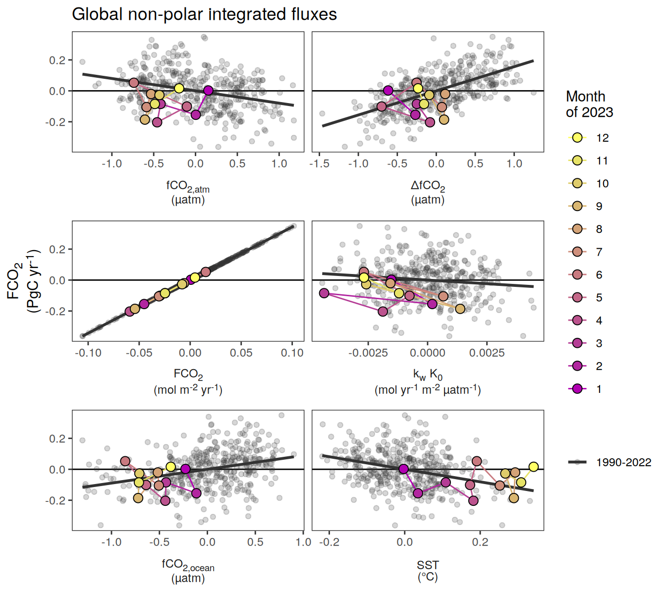
pco2_product_biome_monthly_detrended_anomaly %>%
  filter(!(biome %in% c(key_biomes, "Global non-polar"))) %>%
  pivot_longer(-c(year, month, biome, fgco2_int))  %>%
  filter(name %in% c("temperature", "chl", "dfco2", "kw_sol")) %>% 
  group_split(name) %>%
  head(1) %>%
  map(
    ~ ggplot(data = .x,
             aes(value, fgco2_int)) +
      geom_hline(yintercept = 0) +
      geom_point(
        data = . %>% filter(year != 2023),
        aes(col = paste(min(year), max(year), sep = "-")),
        alpha = 0.2
      ) +
      geom_smooth(
        data = . %>% filter(year != 2023),
        aes(col = paste(min(year), max(year), sep = "-")),
        method = "lm",
        se = FALSE,
        fullrange = TRUE
      )  +
      scale_color_grey(name = "") +
      new_scale_color() +
      geom_path(data = . %>% filter(year == 2023),
                aes(col = as.factor(month), group = 1))  +
      geom_point(
        data = . %>% filter(year == 2023),
        aes(fill = as.factor(month)),
        shape = 21,
        size = 3
      )  +
      scale_color_scico_d(
        palette = "buda",
        guide = guide_legend(reverse = TRUE,
                             order = 1),
        name = paste("Month\nof", 2023)
      ) +
      scale_fill_scico_d(
        palette = "buda",
        guide = guide_legend(reverse = TRUE,
                             order = 1),
        name = paste("Month\nof", 2023)
      ) +
      facet_wrap( ~ biome, ncol = 3, scales = "free") +
      labs(
        title = "Biome integrated fluxes",
        y = labels_breaks("fgco2_int")$i_legend_title,
        x = labels_breaks(.x %>% distinct(name))$i_legend_title
      ) +
      theme(axis.title.x = element_markdown(),
            axis.title.y = element_markdown())
  )

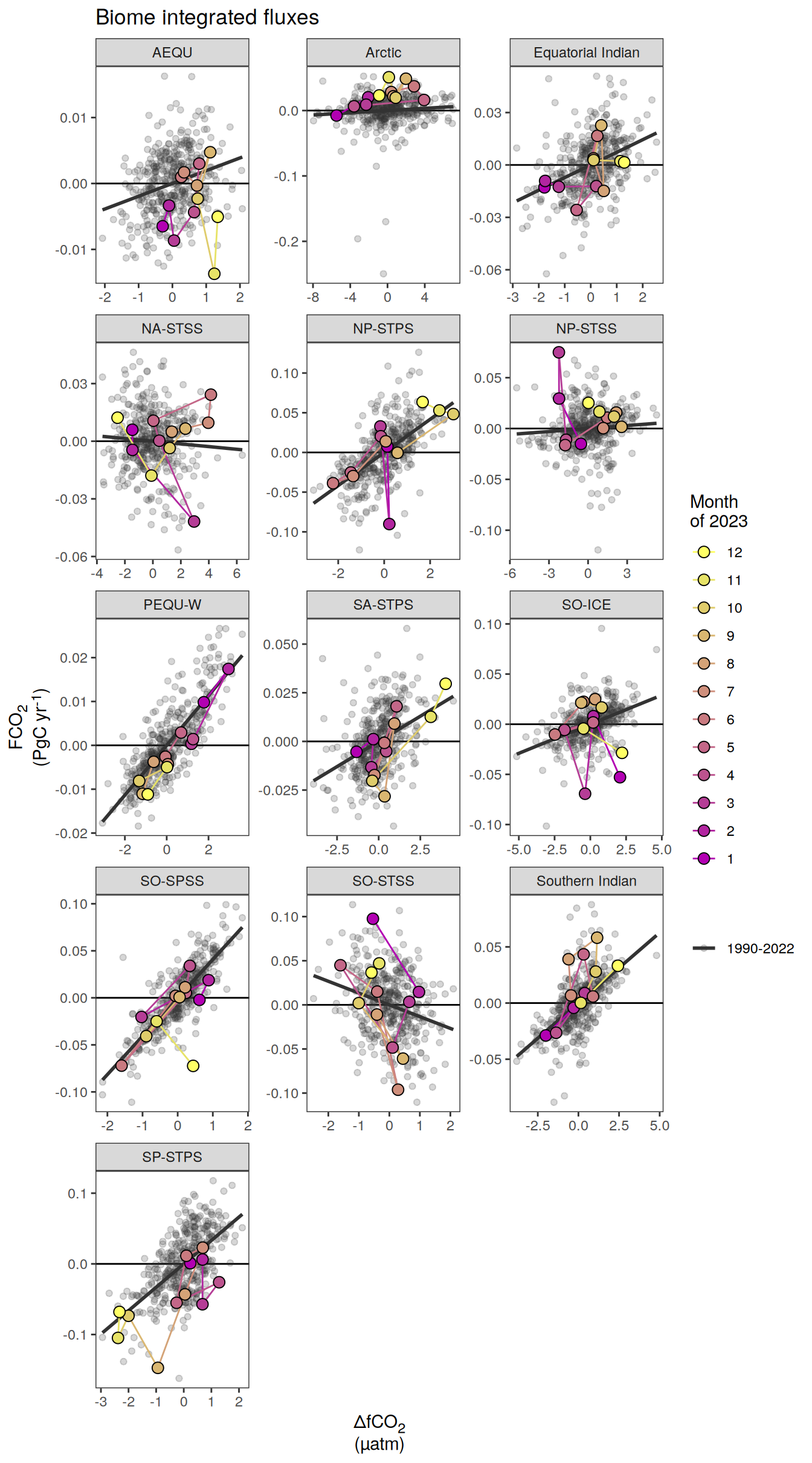
Relative to spread

pco2_product_biome_monthly_detrended_anomaly_spread <-
  pco2_product_biome_monthly_detrended_anomaly %>%
  pivot_longer(-c(month, biome, year)) %>%
  filter(year != 2023) %>%
  group_by(month, biome, name) %>%
  summarise(spread = sd(value, na.rm = TRUE)) %>%
  ungroup()



pco2_product_biome_monthly_detrended_anomaly_relative <-
  full_join(
    pco2_product_biome_monthly_detrended_anomaly_spread,
    pco2_product_biome_monthly_detrended_anomaly %>%
      pivot_longer(-c(month, biome, year))
  )

pco2_product_biome_monthly_detrended_anomaly_relative <-
  pco2_product_biome_monthly_detrended_anomaly_relative %>%
  mutate(value = value / spread) %>%
  select(-spread) %>%
  pivot_wider() %>%
  pivot_longer(-c(month, biome, year, fgco2_int))



pco2_product_biome_monthly_detrended_anomaly_relative %>%
  filter(name %in% c("temperature", "chl", "dfco2", "kw_sol")) %>% 
  group_split(name) %>%
  head(1) %>%
  map(
    ~ ggplot(data = .x,
             aes(value, fgco2_int)) +
      geom_vline(xintercept = 0) +
      geom_hline(yintercept = 0) +
      geom_point(
        data = . %>% filter(year != 2023),
        aes(col = paste(min(year), max(year), sep = "-")),
        alpha = 0.2
      ) +
      geom_smooth(
        data = . %>% filter(year != 2023),
        aes(col = paste(min(year), max(year), sep = "-")),
        method = "lm",
        se = FALSE,
        fullrange = TRUE
      )  +
      scale_color_grey(name = "") +
      new_scale_color() +
      geom_path(data = . %>% filter(year == 2023),
                aes(col = as.factor(month), group = 1))  +
      geom_point(
        data = . %>% filter(year == 2023),
        aes(fill = as.factor(month)),
        shape = 21,
        size = 3
      )  +
      scale_color_scico_d(
        palette = "buda",
        guide = guide_legend(reverse = TRUE,
                             order = 1),
        name = paste("Month\nof", 2023)
      ) +
      scale_fill_scico_d(
        palette = "buda",
        guide = guide_legend(reverse = TRUE,
                             order = 1),
        name = paste("Month\nof", 2023)
      ) +
      facet_wrap( ~ biome, ncol = 3) +
      coord_fixed() +
      labs(
        title = "Biome integrated fluxes normalized to spread",
        y = str_split_i(labels_breaks("fgco2_int")$i_legend_title, "<br>", i = 1),
        x = str_split_i(labels_breaks(.x %>% distinct(name))$i_legend_title, "<br>", i = 1)
      ) +
      theme(axis.title.x = element_markdown(),
            axis.title.y = element_markdown())
  )

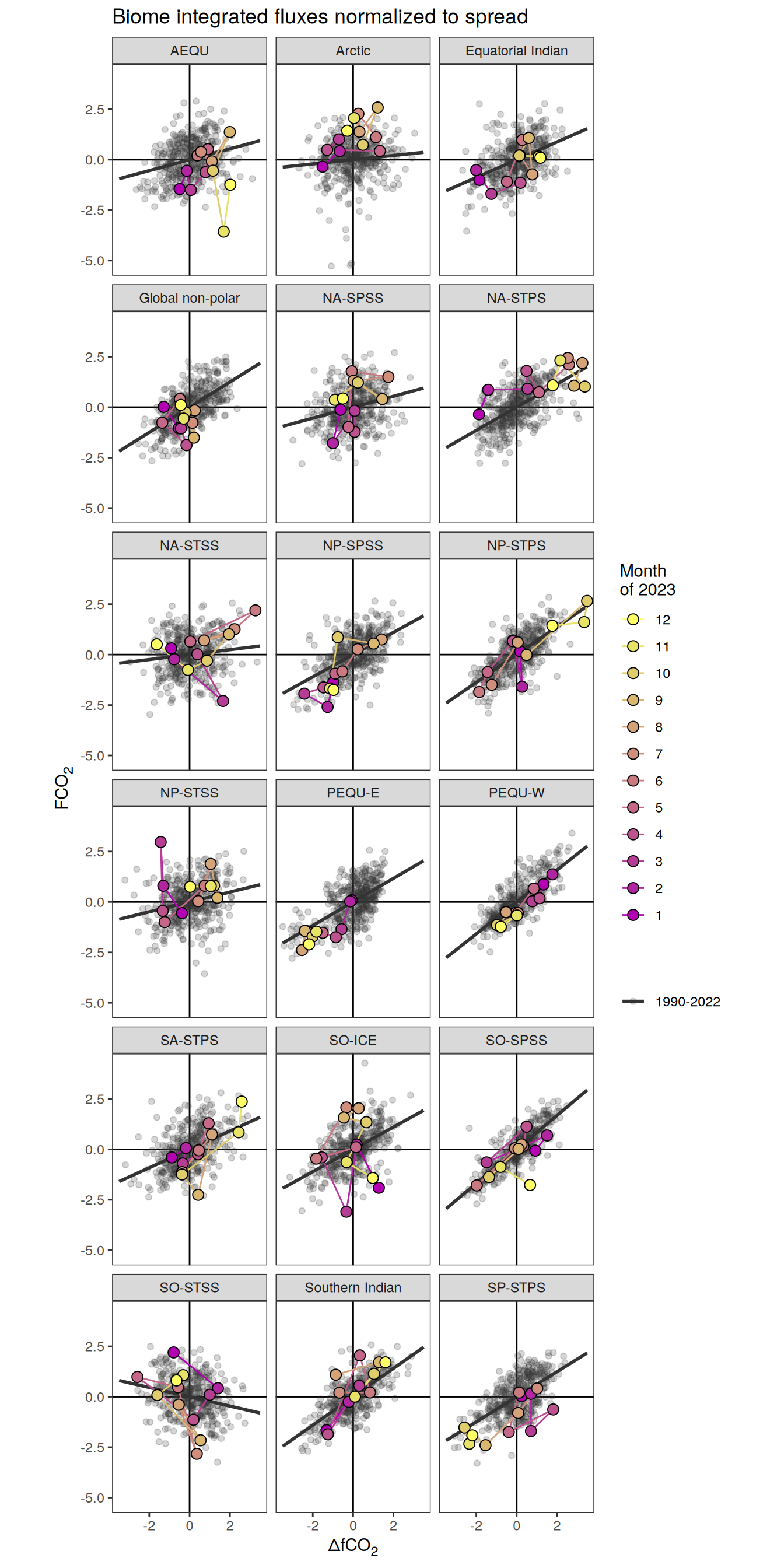
fCO2 decomposition

biome_mask <-
  bind_rows(
    biome_mask,
    biome_mask %>% 
      filter(!str_detect(biome, "SO-SPSS|SO-ICE|Arctic")) %>% 
      mutate(biome = "Global non-polar")
  )

pco2_product_biome_monthly_fCO2_decomposition <-
  full_join(pco2_product_map_monthly_fCO2_decomposition,
            biome_mask,
            relationship = "many-to-many") %>% 
  group_by(year, month, biome, name) %>% 
  summarise(resid = mean(resid, na.rm = TRUE)) %>% 
  ungroup() %>% 
  drop_na()


pco2_product_biome_annual_fCO2_decomposition <-
  pco2_product_biome_monthly_fCO2_decomposition %>%
  group_by(year, biome, name) %>%
  summarise(resid = mean(resid)) %>%
  ungroup()


pco2_product_biome_monthly_fCO2_decomposition %>%
  filter(biome %in% c("Global non-polar", key_biomes)) %>%
  p_season(title  = paste("Anomalies from predicted monthly mean"))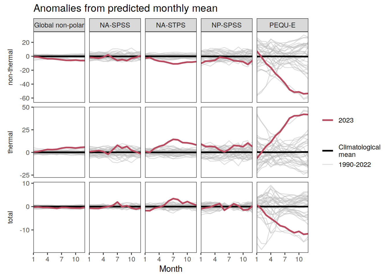

Flux attribution

Seasonal

pco2_product_biome_monthly_flux_attribution <-
  full_join(pco2_product_map_monthly_flux_attribution,
            biome_mask,
            relationship = "many-to-many") %>% 
  group_by(year, month, biome, name) %>% 
  summarise(resid = mean(resid, na.rm = TRUE)) %>% 
  ungroup() %>% 
  drop_na()

pco2_product_biome_monthly_flux_attribution_total <-
  full_join(pco2_product_map_monthly_anomaly %>% 
              filter(name == "fgco2") %>% 
              mutate(name = "resid_fgco2"),
            biome_mask,
            relationship = "many-to-many") %>% 
  group_by(year, month, biome, name) %>% 
  summarise(resid = mean(resid, na.rm = TRUE)) %>% 
  ungroup() %>% 
  drop_na()

pco2_product_biome_monthly_flux_attribution <-
  bind_rows(
    pco2_product_biome_monthly_flux_attribution,
    pco2_product_biome_monthly_flux_attribution_total
  )


pco2_product_biome_annual_flux_attribution <-
  pco2_product_biome_monthly_flux_attribution %>%
  group_by(year, biome, name) %>%
  summarise(resid = mean(resid)) %>%
  ungroup()


pco2_product_biome_monthly_flux_attribution %>%
  filter(year == 2023,
         biome %in% c("Global non-polar", key_biomes)) %>%
  ggplot() +
  geom_hline(yintercept = 0) +
  geom_path(
    aes(month, resid)
  ) +
  geom_point(
    aes(month, resid),
    shape = 21,
    alpha = 0.5,
    col = "grey30"
  ) +
  scale_y_continuous(breaks = seq(-10,10,0.2)) +
  scale_x_continuous(position = "top", breaks = seq(1,12,3)) +
  labs(y = labels_breaks(unique("fgco2"))$i_legend_title) +
  facet_grid(biome ~ name,
             labeller = labeller(name = x_axis_labels),
             scales = "free_y",
             space = "free_y", 
             switch = "x") +
  theme(
    legend.title = element_blank(),
    axis.title.y = element_markdown(),
    strip.text.x.bottom = element_markdown(),
    strip.placement = "outside",
    strip.background.x = element_blank(),
    legend.position = "top"
  )

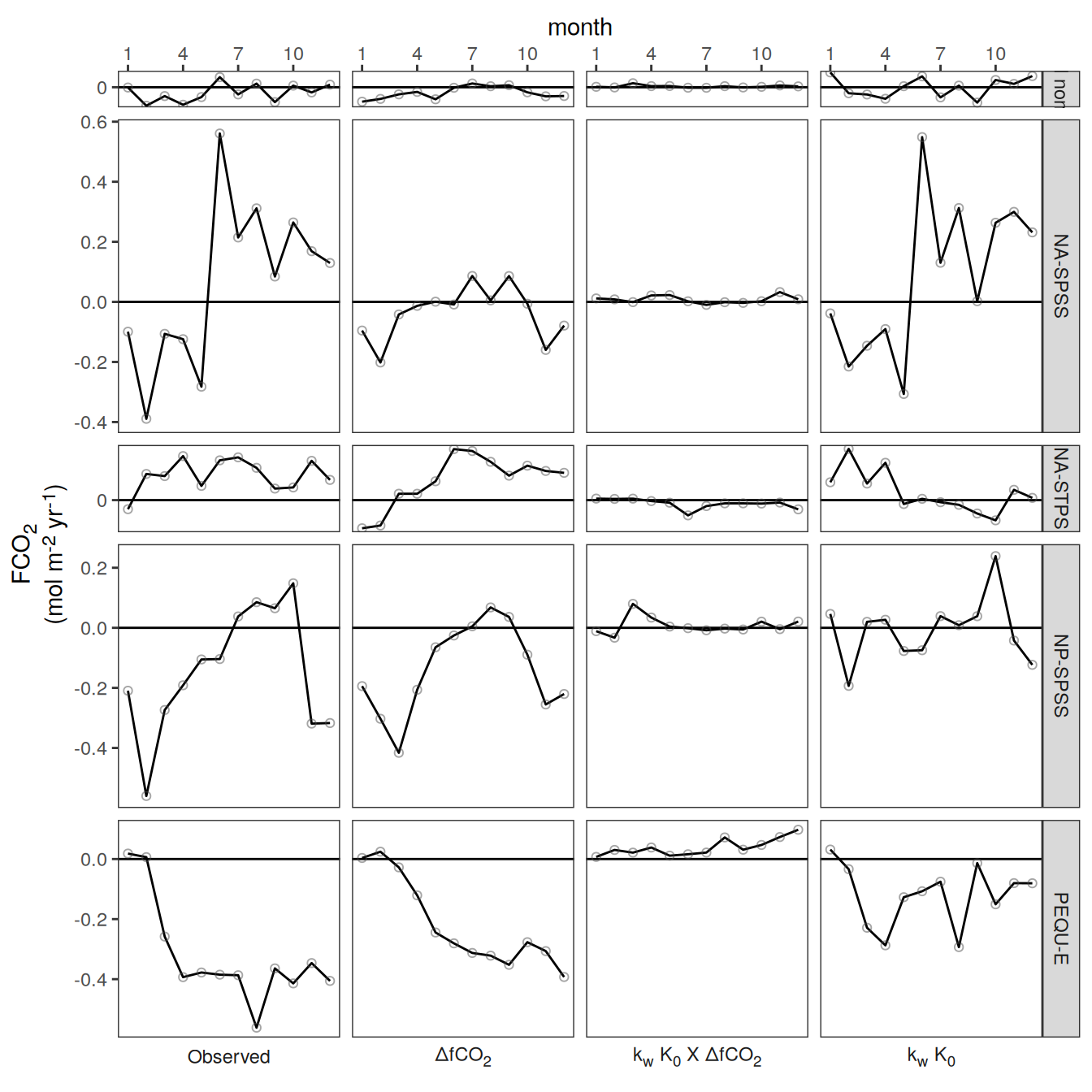
pco2_product_biome_monthly_flux_attribution %>%
  filter(biome %in% c("Global non-polar", key_biomes)) %>%
  p_season(title  = paste("Anomalies from predicted monthly mean"))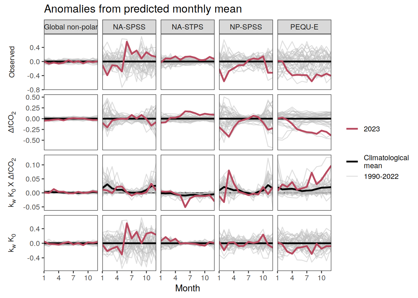

Annual

pco2_product_biome_annual_flux_attribution <-
  full_join(
    pco2_product_biome_annual_flux_attribution %>%
      filter(year == 2023) %>%
      select(-year),
    pco2_product_biome_annual_flux_attribution %>%
      filter(year != 2023) %>%
      group_by(biome, name) %>%
      summarise(resid_mean = mean(abs(resid))) %>%
      ungroup()
  )

# pco2_product_biome_annual_flux_attribution %>%
#   filter(biome %in% c("Global non-polar", key_biomes)) %>%
#   mutate(product == "pco2 product") %>%
#   group_split(product) %>%
#   # head(1) %>%
#   map(
#     ~ ggplot(data = .x) +
#       geom_col(aes("x", resid),
#                position = "dodge2") +
#       geom_col(
#         aes(
#           "x",
#           resid_mean * sign(resid),
#           col = paste0("Mean\nexcl.",2023)
#         ),
#         position = "dodge2",
#         fill = "transparent"
#       ) +
#       labs(y = labels_breaks(unique("fgco2"))$i_legend_title,
#            title = .x$biome) +
#       facet_grid(
#         biome~name,
#         labeller = labeller(name = x_axis_labels),
#         switch = "x"
#       ) +
#       scale_color_grey() +
#       theme(
#         legend.title = element_blank(),
#         axis.text.x = element_blank(),
#         axis.ticks.x = element_blank(),
#         axis.title.x = element_blank(),
#         axis.title.y = element_markdown(),
#         strip.text.x.bottom = element_markdown(),
#         strip.placement = "outside",
#         strip.background.x = element_blank(),
#         legend.position = "top"
#       )
#   )

pco2_product_biome_annual_flux_attribution %>%
  write_csv(
    paste0(
      "../data/",
      "NIES-ML3_GCB",
      "_",
      "2023",
      "_biome_annual_flux_attribution.csv"
    )
  )

pco2_product_biome_monthly_flux_attribution %>%
  write_csv(
    paste0(
      "../data/",
      "NIES-ML3_GCB",
      "_",
      "2023",
      "_biome_monthly_flux_attribution.csv"
    )
  )

pco2_product_biome_annual_fCO2_decomposition %>%
  write_csv(
    paste0(
      "../data/",
      "NIES-ML3_GCB",
      "_",
      "2023",
      "_biome_annual_fCO2_decomposition.csv"
    )
  )

pco2_product_biome_monthly_fCO2_decomposition %>%
  write_csv(
    paste0(
      "../data/",
      "NIES-ML3_GCB",
      "_",
      "2023",
      "_biome_monthly_fCO2_decomposition.csv"
    )
  )

rm(
  pco2_product_biome_annual_flux_attribution,
  pco2_product_biome_monthly_flux_attribution,
  pco2_product_biome_annual_fCO2_decomposition,
  pco2_product_biome_monthly_fCO2_decomposition
)

gc()

Zonal mean sections

The following analysis is available for GOBMs only.

Annual means

2023 anomaly

pco2_product_zonal_mean_annual <-   pco2_product_zonal_mean %>%
  pivot_longer(-c(region, depth, lat, time, year, month)) %>%
  group_by(region, lat, depth, year, name) %>%
  summarise(value = mean(value)) %>%
  ungroup() %>%
  drop_na() %>%
  mutate(region = str_to_title(region))

pco2_product_zonal_mean_annual_anomaly <-
  pco2_product_zonal_mean_annual %>% 
  anomaly_determination(region, lat, depth)

pco2_product_zonal_mean_annual_anomaly %>%
  filter(year == 2023) %>%
  group_split(name) %>%
  # head(3) %>%
  map(
    ~ ggplot(data = .x) +
      geom_contour_filled(aes(lat, depth, z = resid)) +
      scale_fill_discrete_divergingx(name = labels_breaks(.x %>% distinct(name))$i_legend_title) +
      guides(fill = guide_colorsteps(
        barheight = unit(8, "cm"),
        show.limits = TRUE
      )) +
      scale_y_continuous(trans = trans_reverser("sqrt"),
                         breaks = c(50,100,200,400)) +
      scale_x_continuous(breaks = seq(-100, 100, 20)) +
      coord_cartesian(expand = 0) +
      facet_wrap( ~ region, ncol = 1) +
      labs(y = "Depth (m)") +
      theme(legend.title = element_markdown())
  )

pco2_product_zonal_mean_annual_anomaly %>%
  write_csv(
    paste0(
      "../data/",
      "NIES-ML3_GCB",
      "_",
      "2023",
      "_zonal_mean_sections_annual.csv"
    )
  )

Biome profiles

The following analysis is available for GOBMs only.

Annual means

2023 anomaly

pco2_product_profiles_annual <-   pco2_product_profiles %>%
  pivot_longer(-c(biome, depth, time, year, month)) %>%
  group_by(biome, depth, year, name) %>%
  summarise(value = mean(value)) %>%
  ungroup() %>%
  drop_na()

pco2_product_profiles_annual_anomaly <-
  pco2_product_profiles_annual %>% 
  anomaly_determination(biome, depth)

pco2_product_profiles_annual_anomaly %>%
  group_split(name) %>%
  # head(1) %>%
  map(
    ~ ggplot(data = .x) +
      geom_path(aes(resid, depth, group = year), col = "grey30", alpha = 0.5) +
      geom_path(data = .x %>% filter(year == 2023),
                aes(resid, depth, col = as.factor(year)),
                linewidth = 1) +
      scale_y_continuous(trans = trans_reverser("sqrt"),
                         breaks = c(50,100,200,400)) +
      facet_wrap( ~ biome) +
      labs(y = "Depth (m)",
           x = labels_breaks(.x %>% distinct(name))$i_legend_title) +
      theme(legend.title = element_blank(),
            axis.title.x = element_markdown())
  )

pco2_product_profiles_annual_anomaly %>%
  write_csv(
    paste0(
      "../data/",
      "NIES-ML3_GCB",
      "_",
      "2023",
      "_profiles_annual.csv"
    )
  )

Monthly means

2023 anomaly

pco2_product_profiles_monthly <-   pco2_product_profiles %>%
  pivot_longer(-c(biome, depth, time, year, month)) %>%
  group_by(biome, depth, year, month, name) %>%
  summarise(value = mean(value)) %>%
  ungroup() %>%
  drop_na()

pco2_product_profiles_monthly_anomaly <-
  pco2_product_profiles_monthly %>% 
  anomaly_determination(biome, depth, month)

pco2_product_profiles_monthly_anomaly %>%
  filter(year == 2023) %>% 
  group_split(name) %>%
  # head(1) %>%
  map(
    ~ ggplot(data = .x) +
      geom_vline(xintercept = 0) +
      geom_path(aes(resid, depth, col = as.factor(month)),
                linewidth = 1) +
      scale_color_scico_d(palette = "hawaii") +
      scale_y_continuous(trans = trans_reverser("sqrt"),
                         breaks = c(50, 100, 200, 400)) +
      facet_wrap(~ biome,
                 scales = "free_x") +
      labs(y = "Depth (m)",
           x = labels_breaks(.x %>% distinct(name))$i_legend_title) +
      theme(legend.title = element_blank(),
            axis.title.x = element_markdown())
  )

pco2_product_profiles_monthly_anomaly %>%
  write_csv(
    paste0(
      "../data/",
      "NIES-ML3_GCB",
      "_",
      "2023",
      "_profiles_monthly.csv"
    )
  )

Session information

sessionInfo()

R version 4.4.2 (2024-10-31)
Platform: x86_64-pc-linux-gnu
Running under: openSUSE Leap 15.6

Matrix products: default
BLAS/LAPACK: /usr/local/OpenBLAS-0.3.28/lib/libopenblas_haswellp-r0.3.28.so;  LAPACK version 3.12.0

locale:
 [1] LC_CTYPE=en_US.UTF-8       LC_NUMERIC=C              
 [3] LC_TIME=en_US.UTF-8        LC_COLLATE=en_US.UTF-8    
 [5] LC_MONETARY=en_US.UTF-8    LC_MESSAGES=en_US.UTF-8   
 [7] LC_PAPER=en_US.UTF-8       LC_NAME=C                 
 [9] LC_ADDRESS=C               LC_TELEPHONE=C            
[11] LC_MEASUREMENT=en_US.UTF-8 LC_IDENTIFICATION=C       

time zone: Europe/Zurich
tzcode source: system (glibc)

attached base packages:
[1] stats     graphics  grDevices utils     datasets  methods   base     

other attached packages:
 [1] ggh4x_0.3.0         scales_1.3.0        cmocean_0.3-2      
 [4] ggtext_0.1.2        broom_1.0.7         khroma_1.14.0      
 [7] ggnewscale_0.5.0    seacarb_3.3.3       SolveSAPHE_2.1.0   
[10] oce_1.8-3           gsw_1.2-0           stars_0.6-7        
[13] abind_1.4-8         terra_1.8-5         sf_1.0-19          
[16] rnaturalearth_1.0.1 geomtextpath_0.1.4  colorspace_2.1-1   
[19] marelac_2.1.11      shape_1.4.6.1       ggforce_0.4.2      
[22] metR_0.16.0         scico_1.5.0         patchwork_1.3.0    
[25] collapse_2.0.18     lubridate_1.9.3     forcats_1.0.0      
[28] stringr_1.5.1       dplyr_1.1.4         purrr_1.0.2        
[31] readr_2.1.5         tidyr_1.3.1         tibble_3.2.1       
[34] ggplot2_3.5.1       tidyverse_2.0.0     workflowr_1.7.1    

loaded via a namespace (and not attached):
 [1] DBI_1.2.3               rlang_1.1.4             magrittr_2.0.3         
 [4] git2r_0.35.0            e1071_1.7-16            compiler_4.4.2         
 [7] mgcv_1.9-1              getPass_0.2-4           systemfonts_1.1.0      
[10] callr_3.7.6             vctrs_0.6.5             pkgconfig_2.0.3        
[13] crayon_1.5.3            fastmap_1.2.0           backports_1.5.0        
[16] ncmeta_0.4.0            labeling_0.4.3          utf8_1.2.4             
[19] promises_1.3.2          rmarkdown_2.29          markdown_1.13          
[22] tzdb_0.4.0              ps_1.8.1                bit_4.5.0              
[25] xfun_0.49               cachem_1.1.0            jsonlite_1.8.9         
[28] later_1.4.1             tweenr_2.0.3            parallel_4.4.2         
[31] R6_2.5.1                RColorBrewer_1.1-3      bslib_0.8.0            
[34] stringi_1.8.4           jquerylib_0.1.4         Rcpp_1.0.13-1          
[37] knitr_1.49              Matrix_1.7-1            splines_4.4.2          
[40] httpuv_1.6.15           timechange_0.3.0        tidyselect_1.2.1       
[43] RNetCDF_2.9-2           rstudioapi_0.17.1       yaml_2.3.10            
[46] codetools_0.2-20        processx_3.8.4          lattice_0.22-6         
[49] withr_3.0.2             evaluate_1.0.1          rnaturalearthdata_1.0.0
[52] units_0.8-5             proxy_0.4-27            polyclip_1.10-7        
[55] xml2_1.3.6              pillar_1.9.0            whisker_0.4.1          
[58] CFtime_1.4.1            KernSmooth_2.23-24      checkmate_2.3.2        
[61] generics_0.1.3          vroom_1.6.5             rprojroot_2.0.4        
[64] hms_1.1.3               commonmark_1.9.2        munsell_0.5.1          
[67] class_7.3-22            glue_1.8.0              tools_4.4.2            
[70] data.table_1.16.2       fs_1.6.5                grid_4.4.2             
[73] nlme_3.1-166            cli_3.6.3               textshaping_0.4.0      
[76] fansi_1.0.6             viridisLite_0.4.2       gtable_0.3.6           
[79] sass_0.4.9              digest_0.6.37           classInt_0.4-10        
[82] farver_2.1.2            memoise_2.0.1           htmltools_0.5.8.1      
[85] lifecycle_1.0.4         httr_1.4.7              here_1.0.1             
[88] gridtext_0.1.5          bit64_4.5.2             MASS_7.3-61