pCO2 product synopsis 2023 GCB
Jens Daniel Müller
26 June, 2025
Last updated: 2025-06-26
Checks: 7 0
Knit directory:
heatwave_co2_flux_2023/analysis/
This reproducible R Markdown analysis was created with workflowr (version 1.7.1). The Checks tab describes the reproducibility checks that were applied when the results were created. The Past versions tab lists the development history.
Great! Since the R Markdown file has been committed to the Git repository, you know the exact version of the code that produced these results.
Great job! The global environment was empty. Objects defined in the global environment can affect the analysis in your R Markdown file in unknown ways. For reproduciblity it’s best to always run the code in an empty environment.
The command set.seed(20240307) was run prior to running
the code in the R Markdown file. Setting a seed ensures that any results
that rely on randomness, e.g. subsampling or permutations, are
reproducible.
Great job! Recording the operating system, R version, and package versions is critical for reproducibility.
Nice! There were no cached chunks for this analysis, so you can be confident that you successfully produced the results during this run.
Great job! Using relative paths to the files within your workflowr project makes it easier to run your code on other machines.
Great! You are using Git for version control. Tracking code development and connecting the code version to the results is critical for reproducibility.
The results in this page were generated with repository version 7ab307f. See the Past versions tab to see a history of the changes made to the R Markdown and HTML files.
Note that you need to be careful to ensure that all relevant files for
the analysis have been committed to Git prior to generating the results
(you can use wflow_publish or
wflow_git_commit). workflowr only checks the R Markdown
file, but you know if there are other scripts or data files that it
depends on. Below is the status of the Git repository when the results
were generated:
Ignored files:
    Ignored:    .Rhistory
    Ignored:    .Rproj.user/
    Ignored:    data
    Ignored:    output/

Unstaged changes:
    Modified:   analysis/child/pCO2_product_synopsis.Rmd
    Modified:   analysis/mhw_stats.Rmd
    Modified:   analysis/pco2_product_mapping_skill.Rmd
    Modified:   code/Workflowr_project_managment.R
Note that any generated files, e.g. HTML, png, CSS, etc., are not included in this status report because it is ok for generated content to have uncommitted changes.
These are the previous versions of the repository in which changes were
made to the R Markdown
(analysis/pco2_product_synopsis_2023_GCB.Rmd) and HTML
(docs/pco2_product_synopsis_2023_GCB.html) files. If you’ve
configured a remote Git repository (see ?wflow_git_remote),
click on the hyperlinks in the table below to view the files as they
were in that past version.
| File | Version | Author | Date | Message |
|---|---|---|---|---|
| html | 7ab307f | jens-daniel-mueller | 2025-06-26 | Build site. |
| html | 54966ab | jens-daniel-mueller | 2025-06-25 | Build site. |
| html | 265b0a8 | jens-daniel-mueller | 2025-06-06 | Build site. |
| html | 1398df0 | jens-daniel-mueller | 2025-03-14 | Build site. |
| html | c250079 | jens-daniel-mueller | 2025-03-14 | Build site. |
| html | 42ecae0 | jens-daniel-mueller | 2025-03-13 | Build site. |
| html | ff807b1 | jens-daniel-mueller | 2025-03-12 | Build site. |
| html | 3a5d484 | jens-daniel-mueller | 2025-03-11 | Build site. |
| html | b031240 | jens-daniel-mueller | 2025-03-11 | Build site. |
| html | 17f843d | jens-daniel-mueller | 2025-03-10 | Build site. |
| html | fb85a52 | jens-daniel-mueller | 2025-03-10 | Build site. |
| html | ae5b6a4 | jens-daniel-mueller | 2025-03-10 | Build site. |
| html | b9e8f8c | jens-daniel-mueller | 2025-03-10 | Build site. |
| html | 60900ed | jens-daniel-mueller | 2025-03-07 | Build site. |
| html | dd25c0c | jens-daniel-mueller | 2025-03-06 | Build site. |
| html | b76a7c8 | jens-daniel-mueller | 2025-03-04 | Build site. |
| html | 9fe7d3d | jens-daniel-mueller | 2025-03-02 | Build site. |
| Rmd | 481d3cc | jens-daniel-mueller | 2025-03-02 | rerun all analysis |
| html | 9276be7 | jens-daniel-mueller | 2025-03-02 | Build site. |
| html | 417f35d | jens-daniel-mueller | 2025-02-28 | Build site. |
| html | d532d40 | jens-daniel-mueller | 2025-02-28 | Build site. |
| Rmd | f244698 | jens-daniel-mueller | 2025-02-28 | ingest LDEO-HDP |
| html | 518e3d0 | jens-daniel-mueller | 2025-02-27 | Build site. |
| Rmd | 931d9f4 | jens-daniel-mueller | 2025-02-27 | ingest GCB fco2 products |
center <- -160
boundary <- center + 180
target_crs <- paste0("+proj=robin +over +lon_0=", center)
# target_crs <- paste0("+proj=eqearth +over +lon_0=", center)
# target_crs <- paste0("+proj=eqearth +lon_0=", center)
# target_crs <- paste0("+proj=igh_o +lon_0=", center)

worldmap <- ne_countries(scale = 'small',
                         type = 'map_units',
                         returnclass = 'sf')

worldmap <- worldmap %>% st_break_antimeridian(lon_0 = center)
worldmap_trans <- st_transform(worldmap, crs = target_crs)

# ggplot() +
#   geom_sf(data = worldmap_trans)

coastline <- ne_coastline(scale = 'small', returnclass = "sf")
coastline <- st_break_antimeridian(coastline, lon_0 = 200)
coastline_trans <- st_transform(coastline, crs = target_crs)

# ggplot() +
#   geom_sf(data = worldmap_trans, fill = "grey", col="grey") +
#   geom_sf(data = coastline_trans)


bbox <- st_bbox(c(xmin = -180, xmax = 180, ymax = 65, ymin = -78), crs = st_crs(4326))
bbox <- st_as_sfc(bbox)
bbox_trans <- st_break_antimeridian(bbox, lon_0 = center)

bbox_graticules <- st_graticule(
  x = bbox_trans,
  crs = st_crs(bbox_trans),
  datum = st_crs(bbox_trans),
  lon = c(20, 20.001),
  lat = c(-78,65),
  ndiscr = 1e3,
  margin = 0.001
)

bbox_graticules_trans <- st_transform(bbox_graticules, crs = target_crs)
rm(worldmap, coastline, bbox, bbox_trans)

# ggplot() +
#   geom_sf(data = worldmap_trans, fill = "grey", col="grey") +
#   geom_sf(data = coastline_trans) +
#   geom_sf(data = bbox_graticules_trans)

lat_lim <- ext(bbox_graticules_trans)[c(3,4)]*1.002
lon_lim <- ext(bbox_graticules_trans)[c(1,2)]*1.005

# ggplot() +
#   geom_sf(data = worldmap_trans, fill = "grey90", col = "grey90") +
#   geom_sf(data = coastline_trans) +
#   geom_sf(data = bbox_graticules_trans, linewidth = 1) +
#   coord_sf(crs = target_crs,
#            ylim = lat_lim,
#            xlim = lon_lim,
#            expand = FALSE) +
#   theme(
#     panel.border = element_blank(),
#     axis.text = element_blank(),
#     axis.ticks = element_blank()
#   )

latitude_graticules <- st_graticule(
  x = bbox_graticules,
  crs = st_crs(bbox_graticules),
  datum = st_crs(bbox_graticules),
  lon = c(20, 20.001),
  lat = c(-60,-30,0,30,60),
  ndiscr = 1e3,
  margin = 0.001
)

latitude_graticules_trans <- st_transform(latitude_graticules, crs = target_crs)

latitude_labels <- data.frame(lat_label = c("60°N","30°N","Eq.","30°S","60°S"),
                 lat = c(60,30,0,-30,-60)-4, lon = c(35)-c(0,2,4,2,0))

latitude_labels <- st_as_sf(x = latitude_labels,
               coords = c("lon", "lat"),
               crs = "+proj=longlat")

latitude_labels_trans <- st_transform(latitude_labels, crs = target_crs)

# ggplot() +
#   geom_sf(data = worldmap_trans, fill = "grey", col = "grey") +
#   geom_sf(data = coastline_trans) +
#   geom_sf(data = bbox_graticules_trans) +
#   geom_sf(data = latitude_graticules_trans,
#           col = "grey60",
#           linewidth = 0.2) +
#   geom_sf_text(data = latitude_labels_trans,
#                aes(label = lat_label),
#                size = 3,
#                col = "grey60")
pco2_product_list <- c("OceanSODA", "SOM-FFN", "CMEMS", "fco2residual")
# "fCO2-Residual"
gobm_product_list <- c("ETHZ-CESM", "FESOM-REcoM")
files <- list.files(here::here("data/"), pattern = "FESOM-REcoM")
file_types <- str_remove(files, "FESOM-REcoM_2023_")
GCB_products = TRUEpCO2_product_synopsis <-
knitr::knit_expand(
file = here::here("analysis/child/pCO2_product_synopsis.Rmd"),
year_anom = 2023
)Read data
map <-
  read_rds(here::here("data/map.rds"))

key_biomes <-
  read_rds(here::here("data/key_biomes.rds"))

key_biomes <-
key_biomes[!str_detect(key_biomes, "NP")]


biome_mask <-
  read_rds(here::here("data/biome_mask.rds"))

biome_mask_print <-
  biome_mask %>%
  filter(!str_detect(biome, "SO-SPSS|SO-ICE|Arctic")) %>%
  # filter(!str_detect(biome, "SO-ICE|Arctic")) %>%
  select(lon, lat)

region_biomes <-
  read_rds(here::here("data/region_biomes.rds"))
nino_sst <- read_table(here::here("data/nino34sst.txt"))
nino_sst <-
nino_sst %>%
select(year = YR,
month = MON,
resid = ANOM_3)co2_annmean_gl <- read_csv(here::here("data/co2_annmean_gl.csv"),
skip = 37)
co2_gr_gl <- read_csv(here::here("data/co2_gr_gl.csv"),
skip = 43)name_core <- c("fgco2", "fgco2_int", "fgco2_hov",
"sfco2", "atm_fco2",
"dfco2",
# "kw_sol",
"temperature",
# "salinity",
# "dissic", "talk", "sdissic", "stalk", "cstar",
"sdissic_stalk",
"no3", "o2",
"mld", "thetao",
# "so",
"intpp", "chl",
"sfco2_therm","sfco2_nontherm","sfco2_total",
"resid_fgco2_dfco2", "resid_fgco2_kw_sol", "resid_fgco2_dfco2_kw_sol")
all_product_list <- c(pco2_product_list, gobm_product_list)
color_products <- c(
"OceanSODAv2" = "#672933",
"OceanSODA" = "#672933",
"SOM-FFN" = "#d1495b",
"fco2residual" = "#edae49",
"fCO2-Residual" = "#edae49",
"LDEO-HPD" = "#edae49",
"CMEMS" = "#AD8E55",
"ETHZ-CESM" = "#66a182",
"FESOM-REcoM" = "#00798c",
"CSIR-ML6" = "grey10",
"JMA-MLR" = "grey30",
"NIES-ML3" = "grey50",
"UExP-FNN-U" = "grey70"
)
shape_products <- c(
"OceanSODAv2" = 0,
"OceanSODA" = 0,
"SOM-FFN" = 1,
"fco2residual" = 2,
"fCO2-Residual" = 2,
"LDEO-HPD" = 2,
"CMEMS" = 5,
"ETHZ-CESM" = 0,
"FESOM-REcoM" = 1,
"CSIR-ML6" = 6,
"JMA-MLR" = 7,
"NIES-ML3" = 9,
"UExP-FNN-U" = 10
)
warm_color <- "#c33c57"
cold_color <- "#3f6fb3"
trend_color <- "#66a182"
warm_cool_gradient <-
rev(c(
"#61195a",
"#6f185f",
"#8d1e62",
"#aa2960",
"#c33c57",
"#da5351",
"#e77155",
"#f09264",
"#f09264",
"#fbd297",
"#fefefe",
"#c6e8ea",
"#97d4db",
"#79bcd0",
"#5ca2c6",
"#4a88bc",
"#3f6fb3",
"#3e56a2",
"#3c3f82",
"#2f2c5a",
"#272648"
))
# cmocean("balance")(100)for(i_file_type in file_types) {
# print(i_file_type)
# i_file_type <- file_types[1]
files <- list.files(here::here("data"),
pattern = paste(2023, i_file_type, sep = "_"),
full.names = TRUE)
if (GCB_products) {
files <- str_subset(files, paste("_GCB_", paste(gobm_product_list, collapse = "|"), sep = "|"))
files <- str_subset(files, paste(
paste(pco2_product_list, collapse = "|"),
paste(gobm_product_list, collapse = "|"),
sep = "|"
))
} else {
files <- str_subset(files, "_GCB_", negate = TRUE)
}
pco2_product <-
read_csv(files, id = "product")
# pco2_product %>%
# distinct(product)
pco2_product <-
pco2_product %>%
mutate(
product = str_extract(
product,
paste(all_product_list, collapse = "|")
)
)
if (!str_detect(files[1], "slope|_temperature_predict")) {
pco2_product <-
pco2_product %>%
mutate(
name = factor(name, levels = name_core),
product = factor(product, levels = all_product_list)
) %>%
filter(!is.na(name))
} else {
pco2_product <-
pco2_product %>%
mutate(product = factor(product, levels = all_product_list))
}
i_file_type <- str_remove(i_file_type, ".csv")
assign(paste("pco2_product", i_file_type, sep = "_"), pco2_product)
}for(i_file_type in c(
"map_annual_anomaly_temperature_predict.csv",
"biome_annual_anomaly.csv",
"hovmoeller_monthly_anomaly.csv"
)) {
# print(i_file_type)
# i_file_type <- file_types[1]
files <- list.files(
here::here("data"),
pattern = paste("2024", i_file_type, sep = "_"),
full.names = TRUE
)
# if (GCB_products) {
# files <- str_subset(files, paste("_GCB_", paste(gobm_product_list, collapse = "|"), sep = "|"))
# files <- str_subset(files, paste(
# paste(pco2_product_2024_list, collapse = "|"),
# paste(gobm_product_list, collapse = "|"),
# sep = "|"
# ))
# } else {
# files <- str_subset(files, "_GCB_", negate = TRUE)
# }
#
pco2_product_2024 <-
read_csv(files, id = "product")
# pco2_product_2024 %>%
# distinct(product)
pco2_product_2024 <-
pco2_product_2024 %>%
mutate(product = str_extract(product, paste(all_product_list, collapse = "|")))
if (!str_detect(files[1], "slope|_temperature_predict")) {
pco2_product_2024 <-
pco2_product_2024 %>%
mutate(
name = factor(name, levels = name_core),
product = factor(product, levels = all_product_list)
) %>%
filter(!is.na(name))
} else {
pco2_product_2024 <-
pco2_product_2024 %>%
mutate(product = factor(product, levels = all_product_list))
}
i_file_type <- str_remove(i_file_type, ".csv")
assign(paste("pco2_product_2024", i_file_type, sep = "_"),
pco2_product_2024)
}# SOM_FFN_predict_2024_map_annual_anomaly <-
# read_csv(
# "/home/jenmueller/Projects/heatwave_co2_flux_2023/data/SOM-FFN_predict_2024_map_annual_anomaly.csv"
# )
SOM_FFN_predict_2024_map_annual_anomaly_temperature_predict <-
read_csv(
"/home/jenmueller/Projects/heatwave_co2_flux_2023/data/SOM-FFN_predict_2024_map_annual_anomaly_temperature_predict.csv"
)
SOM_FFN_predict_2024_biome_annual_anomaly <-
read_csv(
"/home/jenmueller/Projects/heatwave_co2_flux_2023/data/SOM-FFN_predict_2024_biome_annual_anomaly.csv"
)Define labels and breaks
labels_breaks <- function(i_name) {
  if (i_name == "dco2") {
    i_legend_title <- "ΔpCO<sub>2</sub> anom.<br>(µatm)"
    i_breaks <- c(-Inf, seq(-0.5, 0.5, 0.1), Inf)
  }

  if (i_name == "dfco2") {
    i_legend_title <- "ΔfCO<sub>2</sub> anom.<br>(µatm)"
    i_breaks <- c(-Inf, seq(-12, 12, 3), Inf)
  }

  if (i_name == "atm_co2") {
    i_legend_title <- "pCO<sub>2,atm</sub> anom.<br>(µatm)"
    i_breaks <- c(-Inf, seq(-0.5, 0.5, 0.1), Inf)
  }

  if (i_name == "atm_fco2") {
    i_legend_title <- "fCO<sub>2,atm</sub> anom.<br>(µatm)"
    i_breaks <- c(-Inf, seq(-2, 2, 0.5), Inf)
  }

  if (i_name == "sol") {
    i_legend_title <- "K<sub>0</sub> anom.<br>(mol m<sup>-3</sup> µatm<sup>-1</sup>)"
    i_breaks <- c(-Inf, seq(-0.5, 0.5, 0.1), Inf)
  }

  if (i_name == "kw") {
    i_legend_title <- "k<sub>w</sub> anom.<br>(m yr<sup>-1</sup>)"
    i_breaks <- c(-Inf, seq(-0.5, 0.5, 0.1), Inf)
  }

  if (i_name == "kw_sol") {
    i_legend_title <- "k<sub>w</sub> K<sub>0</sub> anom.<br>(mol yr<sup>-1</sup> m<sup>-2</sup> µatm<sup>-1</sup>)"
    i_breaks <- c(-Inf, seq(-0.015, 0.015, 0.003), Inf)
  }

  if (i_name == "spco2") {
    i_legend_title <- "pCO<sub>2,ocean</sub> anom.<br>(µatm)"
    i_breaks <- c(-Inf, seq(-12, 12, 3), Inf)
  }

  if (i_name == "sfco2") {
    i_legend_title <- "fCO<sub>2,ocean</sub> anom.<br>(µatm)"
    i_breaks <- c(-Inf, seq(-12, 12, 3), Inf)
  }

  if (i_name == "intpp") {
    i_legend_title <- "NPP<sub>int</sub> anom.<br>(mol m<sup>-2</sup> yr<sup>-1</sup>)"
    i_breaks <- c(-Inf, seq(-3, 3, 0.5), Inf)
  }

  if (i_name == "no3") {
    i_legend_title <- "NO<sub>3</sub> anom.<br>(μmol kg<sup>-1</sup>)"
    i_breaks <- c(-Inf, seq(-1.5, 1.5, 0.3), Inf)
  }

  if (i_name == "o2") {
    i_legend_title <- "O<sub>2</sub> anom.<br>(μmol kg<sup>-1</sup>)"
    i_breaks <- c(-Inf, seq(-0.5, 0.5, 0.1), Inf)
  }

  if (i_name == "dissic") {
    i_legend_title <- "DIC anom.<br>(μmol kg<sup>-1</sup>)"
    i_breaks <- c(-Inf, seq(-15, 15, 3), Inf)
  }

  if (i_name == "sdissic") {
    i_legend_title <- "sDIC anom.<br>(μmol kg<sup>-1</sup>)"
    i_breaks <- c(-Inf, seq(-15, 15, 3), Inf)
  }

  if (i_name == "cstar") {
    i_legend_title <- "C* anom.<br>(μmol kg<sup>-1</sup>)"
    i_breaks <- c(-Inf, seq(-0.5, 0.5, 0.1), Inf)
  }

  if (i_name == "talk") {
    i_legend_title <- "TA anom.<br>(μmol kg<sup>-1</sup>)"
    i_breaks <- c(-Inf, seq(-15, 15, 3), Inf)
  }

  if (i_name == "stalk") {
    i_legend_title <- "sTA anom.<br>(μmol kg<sup>-1</sup>)"
    i_breaks <- c(-Inf, seq(-15, 15, 3), Inf)
  }

  if (i_name == "sdissic_stalk") {
    i_legend_title <- "sDIC - sTA anom.<br>(μmol kg<sup>-1</sup>)"
    i_breaks <- c(-Inf, seq(-15, 15, 3), Inf)
  }

  if (i_name == "sfco2_total") {
    i_legend_title <- "total"
    i_breaks <- c(-Inf, seq(-0.5, 0.5, 0.1), Inf)
  }

  if (i_name == "sfco2_therm") {
    i_legend_title <- "thermal"
    i_breaks <- c(-Inf, seq(-0.5, 0.5, 0.1), Inf)
  }

  if (i_name == "sfco2_nontherm") {
    i_legend_title <- "non-thermal"
    i_breaks <- c(-Inf, seq(-0.5, 0.5, 0.1), Inf)
  }

  if (i_name == "fgco2") {
    i_legend_title <- "FCO<sub>2</sub> anom.<br>(mol m<sup>-2</sup> yr<sup>-1</sup>)"
    i_breaks <- c(-Inf, seq(-0.6, 0.6, 0.15), Inf)
  }

  if (i_name == "slope") {
    i_legend_title <- "Slope FCO<sub>2</sub> anom. / SST anom.<br>(mol m<sup>-2</sup> yr<sup>-1</sup> °C<sup>-1</sup>)"
    i_breaks <- c(-Inf, seq(-1, 1, 0.25), Inf)
  }

  if (i_name == "fgco2_predict") {
    i_legend_title <- "FCO<sub>2</sub> anom. pred.<br>(mol m<sup>-2</sup> yr<sup>-1</sup>)"
    i_breaks <- c(-Inf, seq(-0.6, 0.6, 0.15), Inf)
  }

  if (i_name == "fgco2_hov") {
    i_legend_title <- "FCO<sub>2</sub> anom.<br>(PgC deg<sup>-1</sup> yr<sup>-1</sup>)"
    i_breaks <- c(-Inf, seq(-0.5, 0.5, 0.1), Inf)
  }

  if (i_name == "fgco2_int") {
    i_legend_title <- "FCO<sub>2</sub> anom.<br>(PgC yr<sup>-1</sup>)"
    i_breaks <- c(-Inf, seq(-0.5, 0.5, 0.1), Inf)
  }

  if (i_name == "fgco2_predict_int") {
    i_legend_title <- "FCO<sub>2</sub> anom. pred.<br>(PgC yr<sup>-1</sup>)"
    i_breaks <- c(-Inf, seq(-0.5, 0.5, 0.1), Inf)
  }

  if (i_name == "thetao") {
    i_legend_title <- "Temp. anom.<br>(°C)"
    i_breaks <- c(-Inf, seq(-1.6, 1.6, 0.4), Inf)
  }

  if (i_name == "temperature") {
    i_legend_title <- "SST anom.<br>(°C)"
    i_breaks <- c(-Inf, seq(-1.6, 1.6, 0.4), Inf)
  }

  if (i_name == "salinity") {
    i_legend_title <- "SSS anom."
    i_breaks <- c(-Inf, seq(-0.5, 0.5, 0.1), Inf)
  }

  if (i_name == "so") {
    i_legend_title <- "Salinity anom."
    i_breaks <- c(-Inf, seq(-0.5, 0.5, 0.1), Inf)
  }

  if (i_name == "chl") {
    i_legend_title <- "lg(Chl-a) anom.<br>(lg(mg m<sup>-3</sup>))"
    i_breaks <- c(-Inf, seq(-0.2, 0.2, 0.05), Inf)
  }

  if (i_name == "mld") {
    i_legend_title <- "MLD anom.<br>(m)"
    i_breaks <- c(-Inf, seq(-40, 40, 10), Inf)
  }

  if (i_name == "press") {
    i_legend_title <- "pressure<sub>atm</sub> anom.<br>(Pa)"
    i_breaks <- c(-Inf, seq(-0.5, 0.5, 0.1), Inf)
  }

  if (i_name == "wind") {
    i_legend_title <- "Wind anom.<br>(m sec<sup>-1</sup>)"
    i_breaks <- c(-Inf, seq(-0.5, 0.5, 0.1), Inf)
  }

  if (i_name == "SSH") {
    i_legend_title <- "SSH anom.<br>(m)"
    i_breaks <- c(-Inf, seq(-0.5, 0.5, 0.1), Inf)
  }

  if (i_name == "fice") {
    i_legend_title <- "Sea ice anom.<br>(%)"
    i_breaks <- c(-Inf, seq(-0.5, 0.5, 0.1), Inf)
  }


  if (i_name == "resid_fgco2") {
    i_legend_title <-
      "Observed"
    i_breaks <- c(-Inf, seq(-0.5, 0.5, 0.1), Inf)
  }

  if (i_name == "resid_fgco2_dfco2") {
    i_legend_title <-
      "ΔfCO<sub>2</sub> contr."
    i_breaks <- c(-Inf, seq(-0.5, 0.5, 0.1), Inf)
  }

  if (i_name == "resid_fgco2_kw_sol") {
    i_legend_title <-
      "k<sub>w</sub> K<sub>0</sub> contr."
    i_breaks <- c(-Inf, seq(-0.5, 0.5, 0.1), Inf)
  }

  if (i_name == "resid_fgco2_dfco2_kw_sol") {
    i_legend_title <-
      "ΔfCO<sub>2</sub> ⨯ k<sub>w</sub> K<sub>0</sub> contr."
    i_breaks <- c(-Inf, seq(-0.5, 0.5, 0.1), Inf)
  }

  if (i_name == "resid_fgco2_sum") {
    i_legend_title <-
      "∑"
    i_breaks <- c(-Inf, seq(-0.5, 0.5, 0.1), Inf)
  }

  if (i_name == "resid_fgco2_offset") {
    i_legend_title <-
      "Obs. - ∑"
    i_breaks <- c(-Inf, seq(-0.5, 0.5, 0.1), Inf)
  }

  all_labels_breaks <- lst(i_legend_title, i_breaks)

  return(all_labels_breaks)

}

x_axis_labels <-
  c(
    "dco2" = labels_breaks("dco2")$i_legend_title,
    "dfco2" = labels_breaks("dfco2")$i_legend_title,
    "atm_co2" = labels_breaks("atm_co2")$i_legend_title,
    "atm_fco2" = labels_breaks("atm_fco2")$i_legend_title,
    "sol" = labels_breaks("sol")$i_legend_title,
    "kw" = labels_breaks("kw")$i_legend_title,
    "kw_sol" = labels_breaks("kw_sol")$i_legend_title,
    "intpp" = labels_breaks("intpp")$i_legend_title,
    "no3" = labels_breaks("no3")$i_legend_title,
    "o2" = labels_breaks("o2")$i_legend_title,
    "dissic" = labels_breaks("dissic")$i_legend_title,
    "sdissic" = labels_breaks("sdissic")$i_legend_title,
    "cstar" = labels_breaks("cstar")$i_legend_title,
    "talk" = labels_breaks("talk")$i_legend_title,
    "stalk" = labels_breaks("stalk")$i_legend_title,
    "sdissic_stalk" = labels_breaks("sdissic_stalk")$i_legend_title,
    "spco2" = labels_breaks("spco2")$i_legend_title,
    "sfco2" = labels_breaks("sfco2")$i_legend_title,
    "sfco2_total" = labels_breaks("sfco2_total")$i_legend_title,
    "sfco2_therm" = labels_breaks("sfco2_therm")$i_legend_title,
    "sfco2_nontherm" = labels_breaks("sfco2_nontherm")$i_legend_title,
    "fgco2" = labels_breaks("fgco2")$i_legend_title,
    "slope" = labels_breaks("slope")$i_legend_title,
    "fgco2_predict" = labels_breaks("fgco2_predict")$i_legend_title,
    "fgco2_hov" = labels_breaks("fgco2_hov")$i_legend_title,
    "fgco2_int" = labels_breaks("fgco2_int")$i_legend_title,
    "fgco2_predict_int" = labels_breaks("fgco2_predict_int")$i_legend_title,
    "thetao" = labels_breaks("thetao")$i_legend_title,
    "temperature" = labels_breaks("temperature")$i_legend_title,
    "salinity" = labels_breaks("salinity")$i_legend_title,
    "so" = labels_breaks("so")$i_legend_title,
    "chl" = labels_breaks("chl")$i_legend_title,
    "mld" = labels_breaks("mld")$i_legend_title,
    "press" = labels_breaks("press")$i_legend_title,
    "wind" = labels_breaks("wind")$i_legend_title,
    "SSH" = labels_breaks("SSH")$i_legend_title,
    "fice" = labels_breaks("fice")$i_legend_title,
    "resid_fgco2" = labels_breaks("resid_fgco2")$i_legend_title,
    "resid_fgco2_dfco2" = labels_breaks("resid_fgco2_dfco2")$i_legend_title,
    "resid_fgco2_kw_sol" = labels_breaks("resid_fgco2_kw_sol")$i_legend_title,
    "resid_fgco2_dfco2_kw_sol" = labels_breaks("resid_fgco2_dfco2_kw_sol")$i_legend_title,
    "resid_fgco2_sum" = labels_breaks("resid_fgco2_sum")$i_legend_title,
    "resid_fgco2_offset" = labels_breaks("resid_fgco2_offset")$i_legend_title
  )

# create axis labels for absolute values by removing anom.
x_axis_labels_abs <- x_axis_labels
x_axis_labels_abs <- str_replace_all(x_axis_labels_abs, " anom.", "")
names(x_axis_labels_abs) <- names(x_axis_labels)
Functions
Seasonality plots
p_season <- function(df,
                     dim_row = "name",
                     dim_col = "product",
                     title = NULL,
                     var = "resid",
                     scales = "free_y") {

  p <- ggplot(data = df,
              aes(month, !!ensym(var)))

  if(var == "resid"){
      p <- p +
        geom_hline(yintercept = 0, linewidth =0.5)

  }


  p <- p +
      geom_path(data = . %>% filter(year != 2023),
                aes(group = as.factor(year),
                    col = as.factor(paste(min(year), max(year), sep = "-"))),
                alpha = 0.5)+
      geom_path(data = . %>%
                  filter(year != 2023) %>%
                  group_by_at(vars(month, dim_col, dim_row)) %>%
                  summarise(!!ensym(var) := mean(!!ensym(var))),
                aes(col = "Climatological\nmean"),
                linewidth = 0.7) +
    scale_color_manual(values = c("grey60", "grey10"),
                       guide = guide_legend(order = 2,
                                            reverse = TRUE)) +
    new_scale_color()+
    geom_path(data = . %>% filter(year == 2023),
                aes(col = as.factor(year)),
                linewidth = 1.2) +
      scale_color_manual(
        values = warm_color,
        guide = guide_legend(order = 1)
      ) +
      scale_x_continuous(breaks = seq(1, 12, 3), expand = c(0, 0)) +
      labs(title = title,
           x = "Month")

    if(df %>% filter(name == "fgco2") %>% nrow() > 0 & "value" %in% names(df)){

    df_sink <- df %>%
      filter(year == 2023,
             name == "fgco2")

      p <- p +
          geom_point(data = df_sink %>% filter(value < 0),
             aes(shape = "Sink"), fill = "white") +
          geom_point(data = df_sink %>% filter(value >= 0),
             aes(shape = "Source"), fill = "white") +
        scale_shape_manual(values = c(25,24))

  }


  if (!(is.null(dim_col))) {
    p <- p +
      facet_grid2(
        as.formula(paste(dim_row, "~", dim_col)),
        scales = scales,
        # independent = "y",
        labeller = labeller(name = x_axis_labels),
        switch = "y"
      )


  } else {
    p <- p +
      facet_grid(
        as.formula(paste(dim_row, "~ .")),
        scales = scales,
        # independent = "y",
        labeller = labeller(name = x_axis_labels),
        switch = "y"
      )
  }

  p <- p +
    theme(
      strip.text.y.left = element_markdown(),
      strip.placement = "outside",
      strip.background.y = element_blank(),
      axis.title.y = element_blank(),
      legend.title = element_blank(),
      axis.text.y.right = element_blank()
    )
    # scale_y_continuous(sec.axis = dup_axis())

  p

}
fCO2 decomposition
fco2_decomposition <- function(df, ...) {

  group_by <- quos(...)
  # group_by <- quos(lon, lat, month)
  # group_by <- quos(biome, year, month)

  pco2_product_biome_monthly_fCO2_decomposition <-
    df %>%
    filter(name %in% c("temperature", "sfco2"))

  pco2_product_biome_monthly_fCO2_decomposition <-
    inner_join(
      pco2_product_biome_monthly_fCO2_decomposition %>%
        filter(name == "temperature") %>%
        select(-c(value, fit)) %>%
        pivot_wider(values_from = resid),
      pco2_product_biome_monthly_fCO2_decomposition %>%
        filter(name == "sfco2") %>%
        select(-c(value, resid)) %>%
        pivot_wider(values_from = fit)
    )

  pco2_product_biome_monthly_fCO2_decomposition <-
    pco2_product_biome_monthly_fCO2_decomposition %>%
    mutate(sfco2_therm = (sfco2 * exp(0.0423 * temperature)) - sfco2)


  pco2_product_biome_monthly_fCO2_decomposition <-
    inner_join(
      pco2_product_biome_monthly_fCO2_decomposition,
      df %>%
        filter(name %in% c("sfco2")) %>%
        select(-c(value, fit, name)) %>%
        rename(sfco2_total = resid)
    )


  pco2_product_biome_monthly_fCO2_decomposition <-
    pco2_product_biome_monthly_fCO2_decomposition %>%
    mutate(sfco2_nontherm = sfco2_total - sfco2_therm)

  pco2_product_biome_monthly_fCO2_decomposition <-
    pco2_product_biome_monthly_fCO2_decomposition %>%
    select(-c(temperature, sfco2)) %>%
    pivot_longer(starts_with("sfco2"),
                 values_to = "resid")

}
Flux attribution
flux_attribution <- function(df, ...) {

  group_by <- quos(...)
  # group_by <- quos(lon, lat, month)

  pco2_product_flux_attribution <-
    df %>%
    filter(name %in% c("dfco2", "kw_sol", "fgco2"))


  pco2_product_flux_attribution <-
    inner_join(
      pco2_product_flux_attribution %>%
        select(-c(value, fit)) %>%
        pivot_wider(values_from = resid,
                    names_prefix = "resid_"),
      pco2_product_flux_attribution %>%
        select(-c(value, resid)) %>%
        filter(name != "fgco2") %>%
        pivot_wider(values_from = fit)
    )

    pco2_product_flux_attribution <-
    pco2_product_flux_attribution %>%
    mutate(
      resid_fgco2_dfco2 = resid_dfco2 * kw_sol,
      resid_fgco2_kw_sol = resid_kw_sol * dfco2,
      resid_fgco2_dfco2_kw_sol = resid_dfco2 * resid_kw_sol
      # resid_fgco2_sum = resid_fgco2_dfco2 + resid_fgco2_kw_sol + resid_fgco2_dfco2_kw_sol
    )

  # pco2_product_flux_attribution <-
  #   pco2_product_flux_attribution %>%
  #   mutate(resid_fgco2_offset = resid_fgco2 - resid_fgco2_sum)

  pco2_product_flux_attribution <-
    pco2_product_flux_attribution %>%
    select(product, !!!group_by, starts_with("resid_fgco2")) %>%
    pivot_longer(starts_with("resid_"),
                 values_to = "resid")


  pco2_product_flux_attribution <-
    pco2_product_flux_attribution %>%
    filter(str_detect(name, "dfco2|kw_sol")) %>%
    mutate(name = factor(
      name,
      levels = c(
        "resid_fgco2",
        "resid_fgco2_dfco2",
        "resid_fgco2_kw_sol",
        "resid_fgco2_dfco2_kw_sol",
        "resid_fgco2_sum",
        "resid_fgco2_offset"
      )
    ))

}
Robinson map
bbox <- st_bbox(c(xmin = -180, xmax = 180, ymax = 76, ymin = -54), crs = st_crs(4326))
# bbox <- st_bbox(c(xmin = -180, xmax = 180, ymax = 85, ymin = -80), crs = st_crs(4326))
bbox <- st_as_sfc(bbox)
bbox_trans <- st_break_antimeridian(bbox, lon_0 = center)

bbox_graticules <- st_graticule(
  x = bbox_trans,
  crs = st_crs(bbox_trans),
  datum = st_crs(bbox_trans),
  lon = c(20, 20.001),
  lat = c(-54,76),
  # lat = c(-80,85),
  ndiscr = 1e3,
  margin = 0.001
)

bbox_graticules_trans <- st_transform(bbox_graticules, crs = target_crs)
rm(bbox, bbox_trans)

# ggplot() +
#   geom_sf(data = worldmap_trans, fill = "grey", col="grey") +
#   geom_sf(data = coastline_trans) +
#   geom_sf(data = bbox_graticules_trans)

lat_lim <- ext(bbox_graticules_trans)[c(3,4)]*1.002
lon_lim <- ext(bbox_graticules_trans)[c(1,2)]*1.005


p_map_mdim_robinson <-
  function(df,
           df_uncertainty = NULL,
           dim_row = NULL,
           dim_col = NULL,
           dim_wrap = NULL,
           n_col = NULL,
           var,
           legend_title = NULL,
           breaks = NULL,
           n_labels = 2,
           target_crs = "+proj=robin +over +lon_0=-160",
           col = "divergent",
           col_scale = "warm_cold",
           plot_latitudes = FALSE,
           legend_position = "top") {

    if (is.null(dim_col) & is.null(dim_row) & is.null(dim_wrap)) {
      df_raster <- df %>%
        select(lon, lat, all_of(var)) %>%
        rast(crs = "+proj=longlat")

      df_raster <-
        project(df_raster, target_crs)

      df_tibble <-
        df_raster %>%
        as.data.frame(xy = TRUE, na.rm = FALSE) %>%
        as_tibble() %>%
        rename(lon = x, lat = y) %>%
        drop_na()


    } else {

      # if (!is.null(dim_col) & !is.null(dim_row) & !is.null(dim_wrap)) {
      #   names_sep <- ";"
      # } else {
      #   names_sep <- NULL
      # }

      names_sep <- ";"

      df_raster <- df %>%
        select(lon, lat,
               all_of(c(dim_row, dim_col, dim_wrap)),
               all_of(var)) %>%
        pivot_wider(names_from = all_of(c(dim_row, dim_col, dim_wrap)),
                    values_from = all_of(var),
                    names_sep = names_sep) %>%
        rast(crs = "+proj=longlat")


      df_raster <-
        project(df_raster, target_crs)


      if (length(c(dim_row, dim_col, dim_wrap)) <= 1) {
        names_sep <- NULL
      }

      df_tibble <-
        df_raster %>%
        as.data.frame(xy = TRUE, na.rm = FALSE) %>%
        as_tibble() %>%
        rename(lon = x, lat = y) %>%
        pivot_longer(
          -c(lon, lat),
          names_sep = names_sep,
          names_to = c(dim_row, dim_col, dim_wrap),
          values_to = var
        ) %>%
        drop_na()


    }


    if (is.null(legend_title)) {
      legend_title <- var
    }

    var <- sym(var)

    p_map <- ggplot() +
      geom_raster(data = df_tibble, aes(
        x = lon,
        y = lat,
        fill = cut(!!var, breaks, include.lowest = TRUE)
      ))


    p_map <- p_map +
      geom_sf(data = worldmap_trans %>% select(-name),
              fill = "grey90",
              col = "grey90") +
      geom_sf(data = coastline_trans, linewidth = 0.3) +
      geom_sf(data = bbox_graticules_trans, linewidth = 0.5)

    if (plot_latitudes) {
      p_map <- p_map +
        geom_sf(data = latitude_graticules_trans,
                col = "grey60",
                linewidth = 0.2) +
        geom_sf_text(
          data = latitude_labels_trans,
          aes(label = lat_label),
          size = 3,
          col = "grey60"
        )
    }

    if (!is.null(df_uncertainty)) {
      p_map <- p_map +
        geom_sf(
          data = df_uncertainty %>% filter(signif_single == 0),
          col = "grey60",
          size = 0.05
        )
    }

    p_map <- p_map +
      coord_sf(
        crs = target_crs,
        ylim = lat_lim,
        xlim = lon_lim,
        expand = FALSE
      )

    if (legend_position == "top") {
      p_map <- p_map +
        guides(
          fill = guide_colorsteps(
            barheight = unit(0.3, "cm"),
            barwidth = unit(8, "cm"),
            ticks = TRUE,
            ticks.colour = "grey20",
            frame.colour = "grey20",
            label.position = "top",
            direction = "horizontal"
          )
        ) +
        theme_void() +
        theme(
          legend.margin=margin(t = .1, b = .1, unit='cm'),
          plot.margin = margin(.1,.1,.1,.1,"cm"),
          panel.spacing = unit(.1,"cm"),
          legend.position = "top",
          legend.title.align = 1,
          legend.box.spacing = unit(0.1, "cm"),
          legend.title = element_markdown(halign = 1, lineheight = 1.5)
        )
    }

    if (legend_position == "bottom") {
      p_map <- p_map +
        guides(
          fill = guide_colorsteps(
            barheight = unit(0.3, "cm"),
            barwidth = unit(8, "cm"),
            ticks = TRUE,
            ticks.colour = "grey20",
            frame.colour = "grey20",
            label.position = "bottom",
            direction = "horizontal"
          )
        ) +
        theme_void() +
        theme(
          legend.margin=margin(t = .1, b = .1, unit='cm'),
          plot.margin = margin(.1,.1,.1,.1,"cm"),
          panel.spacing = unit(.1,"cm"),
          legend.position = "bottom",
          legend.title.align = 1,
          legend.box.spacing = unit(0.1, "cm"),
          legend.title = element_markdown(halign = 1, lineheight = 1.5)
        )
    }

    if (legend_position == "right") {
      p_map <- p_map +
        guides(
          fill = guide_colorsteps(
            barheight = unit(6, "cm"),
            barwidth = unit(0.3, "cm"),
            ticks = TRUE,
            ticks.colour = "grey20",
            frame.colour = "grey20",
            label.position = "right",
            direction = "vertical"
          )
        ) +
        theme_void() +
        theme(
          legend.position = "right",
          legend.title.align = 0,
          legend.box.spacing = unit(0.1, "cm"),
          legend.title = element_markdown(halign = 0, lineheight = 1.5)
        )
    }

    if (legend_position == "left") {
      p_map <- p_map +
        guides(
          fill = guide_colorsteps(
            barheight = unit(6, "cm"),
            barwidth = unit(0.3, "cm"),
            ticks = TRUE,
            ticks.colour = "grey20",
            frame.colour = "grey20",
            label.position = "left",
            direction = "vertical"
          )
        ) +
        theme_void() +
        theme(
          legend.position = "left",
          legend.title.align = 0,
          legend.box.spacing = unit(0.1, "cm"),
          legend.title = element_markdown(halign = 0, lineheight = 1.5)
        )
    }

    if (col == "sequential") {
      breaks_test <- breaks[!breaks == Inf]
      breaks_test <- breaks_test[!breaks_test == -Inf]
      breaks_reverse <-
        abs(first(breaks_test)) < abs(last(breaks_test))

      if (breaks_reverse == TRUE) {
        direction_value = 1
        reverse_value = TRUE
      } else{
        direction_value = -1
        reverse_value = FALSE
      }

      if (n_labels == 1) {
        labels <- breaks_test
      } else {
        breaks_test[seq_along(breaks_test) %% 2 == 0] <- ""
        labels <- breaks_test
      }

      if (col_scale %in% c("viridis", "plasma", "cividis")) {
        p_map <- p_map +
          scale_fill_viridis_d(
            drop = FALSE,
            name = legend_title,
            direction = direction_value,
            option = col_scale,
            labels = unname(labels)
          )
      }

    } else {

      breaks_test <- breaks[!breaks == Inf]
      breaks_test <- breaks_test[!breaks_test == -Inf]

      if (n_labels == 1) {
        labels <- breaks_test
      } else {
        breaks_test[seq_along(breaks_test) %% 2 == 0] <- ""
        labels <- breaks_test
      }

      p_map <- p_map +
        scale_fill_gradientn(
          colours = warm_cool_gradient,
          # rescaler = ~ scales::rescale_mid(.x, mid = 0),
          super = ScaleDiscretised,
          name = legend_title,
          labels = unname(labels)
        )
        # colorspace::scale_fill_discrete_divergingx(
        #   palette = "RdBu",
        #   drop = FALSE,
        #   rev = TRUE,
        #   name = legend_title,
        #   labels = unname(labels)
        # )
    }


    if (!(is.null(dim_row) & is.null(dim_col))) {
      if (is.null(dim_col)) {
        dim_col <- "."
      }

      if (is.null(dim_row)) {
        dim_row <- "."
      }

      p_map <- p_map +
        facet_grid(as.formula(paste(dim_row, "~", dim_col)),
                   labeller = labeller(name = x_axis_labels),
                   switch = "y") +
        theme(strip.text.x.top = element_markdown(),
              strip.text.y.left = element_markdown())

    }

    if (!is.null(dim_wrap) & is.null(n_col)) {

      p_map <- p_map +
        facet_wrap(as.formula(paste("~", dim_wrap)))
    }


    if (!(is.null(dim_wrap) & is.null(n_col))) {
      if (dim_wrap == "name") {
        p_map <- p_map +
          facet_wrap(as.formula(paste("~", dim_wrap)),
                     labeller = labeller(name = x_axis_labels),
                     ncol = n_col) +
          theme(strip.text.x.top = element_markdown())
      } else{
        p_map <- p_map +
          facet_wrap(as.formula(paste("~", dim_wrap)), ncol = n_col) +
          theme(strip.text.x.top = element_markdown())
      }
    }

    p_map

  }
Maps
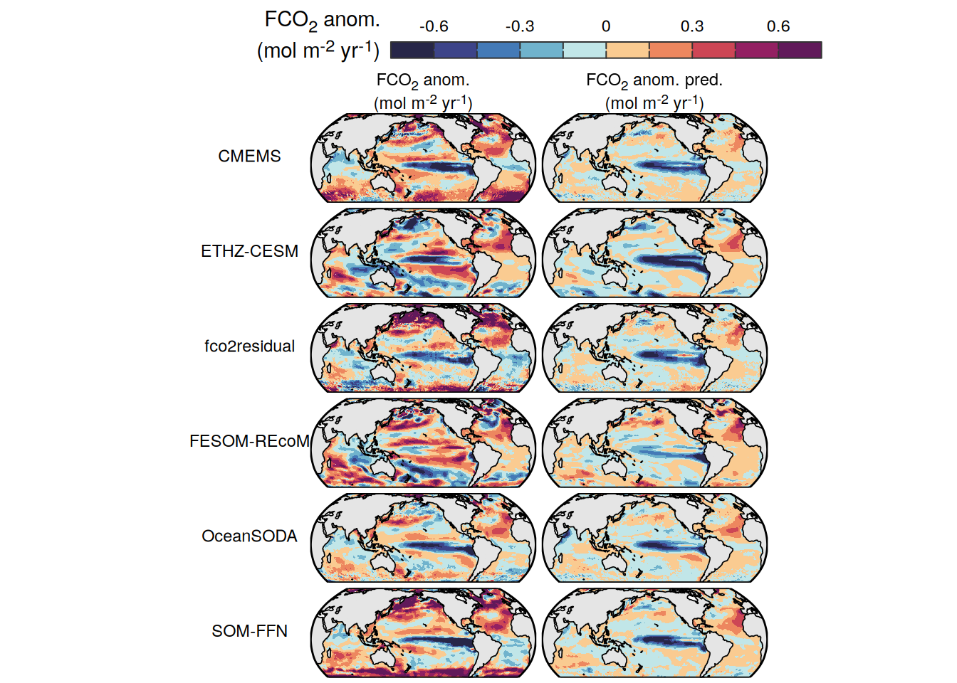
The following maps show the anomalies of each variable in 2023 as provided through the fCO2 product. Anomalies are determined based on the predicted value of a linear regression model fit to the available data from 1990 to 2022.
Maps are first presented as annual means, and than as monthly means. Note that the 2023 predictions for the monthly maps are done individually for each month, such the mean seasonal anomaly from the annual mean is removed.
Note: The increase the computational speed, I regridded all maps to 5X5° grid.
Annual means
2023 anomaly
pco2_product_map_annual_anomaly <-
  inner_join(
    biome_mask_print,
    pco2_product_map_annual_anomaly
  )

pco2_product_map_annual_anomaly %>%
  filter(year == 2023) %>%
  group_split(name) %>%
  # head(1) %>%
  map(
    ~ p_map_mdim_robinson(
      df = .x,
      var = "resid",
      legend_title = labels_breaks(.x %>% distinct(name))$i_legend_title,
      breaks = labels_breaks(.x %>% distinct(name))$i_breaks,
      dim_wrap = "product",
      n_col = 2
    )
  )
[[1]]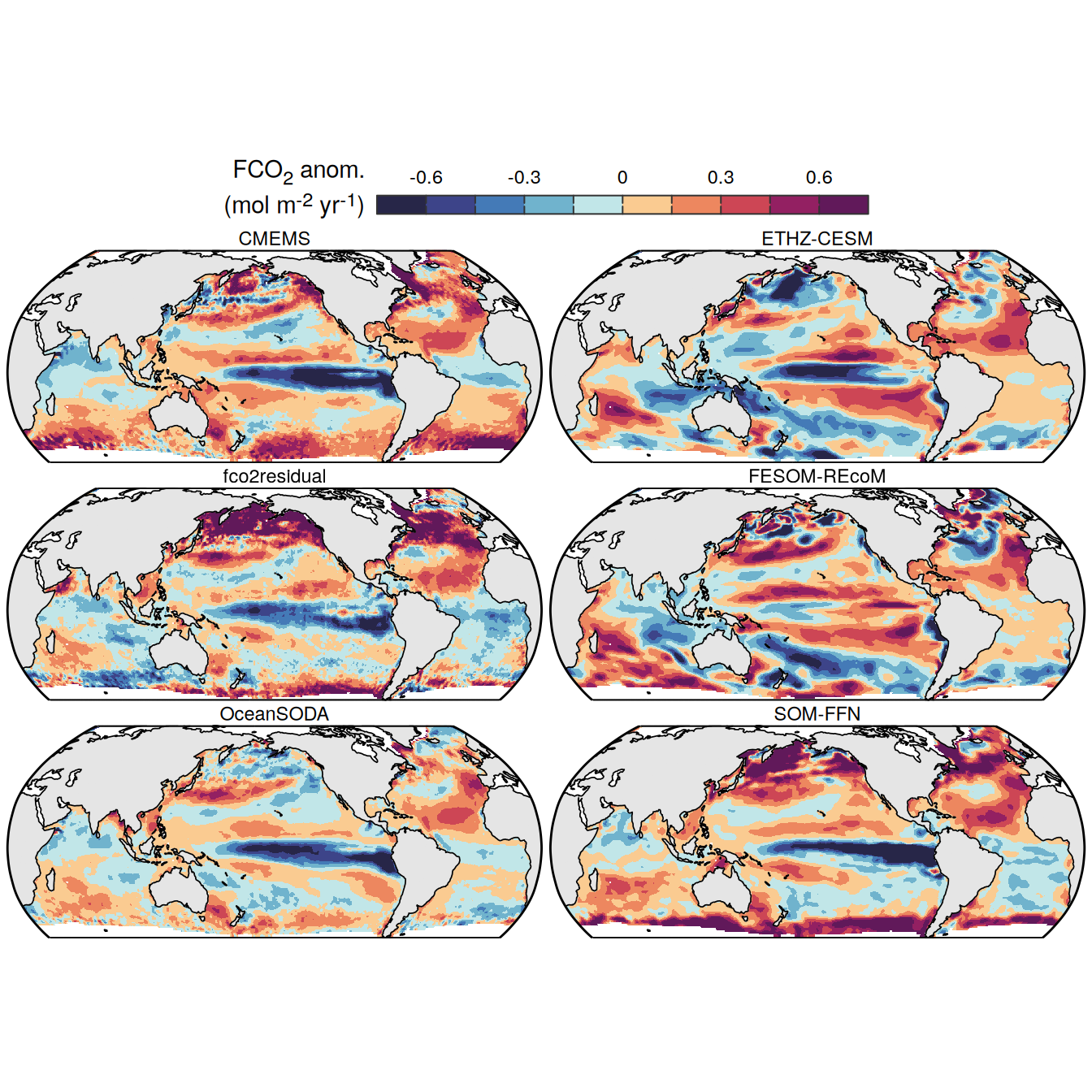
| Version | Author | Date |
|---|---|---|
| 42ecae0 | jens-daniel-mueller | 2025-03-13 |
| 17f843d | jens-daniel-mueller | 2025-03-10 |
| fb85a52 | jens-daniel-mueller | 2025-03-10 |
| ae5b6a4 | jens-daniel-mueller | 2025-03-10 |
| b9e8f8c | jens-daniel-mueller | 2025-03-10 |
| 9fe7d3d | jens-daniel-mueller | 2025-03-02 |
| 9276be7 | jens-daniel-mueller | 2025-03-02 |
| 417f35d | jens-daniel-mueller | 2025-02-28 |
| d532d40 | jens-daniel-mueller | 2025-02-28 |
| 518e3d0 | jens-daniel-mueller | 2025-02-27 |
[[2]]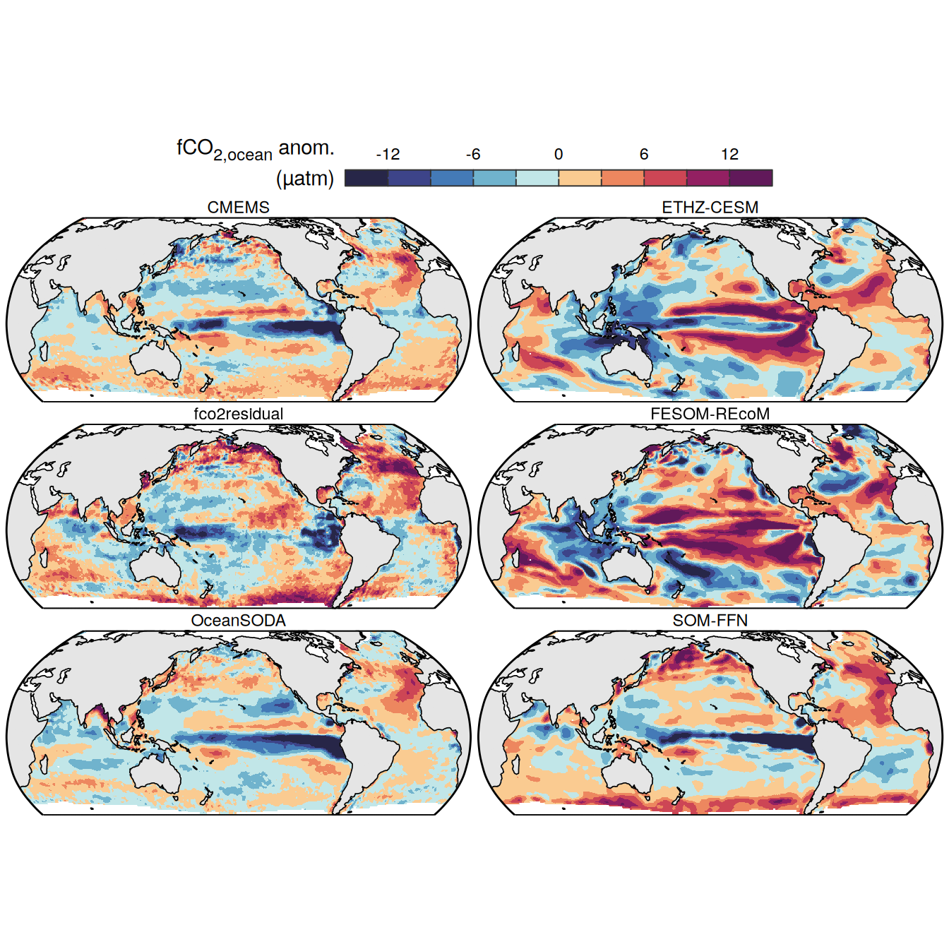
| Version | Author | Date |
|---|---|---|
| 1398df0 | jens-daniel-mueller | 2025-03-14 |
| 17f843d | jens-daniel-mueller | 2025-03-10 |
| fb85a52 | jens-daniel-mueller | 2025-03-10 |
| ae5b6a4 | jens-daniel-mueller | 2025-03-10 |
| b9e8f8c | jens-daniel-mueller | 2025-03-10 |
| 9fe7d3d | jens-daniel-mueller | 2025-03-02 |
| 9276be7 | jens-daniel-mueller | 2025-03-02 |
| 417f35d | jens-daniel-mueller | 2025-02-28 |
| d532d40 | jens-daniel-mueller | 2025-02-28 |
| 518e3d0 | jens-daniel-mueller | 2025-02-27 |
[[3]]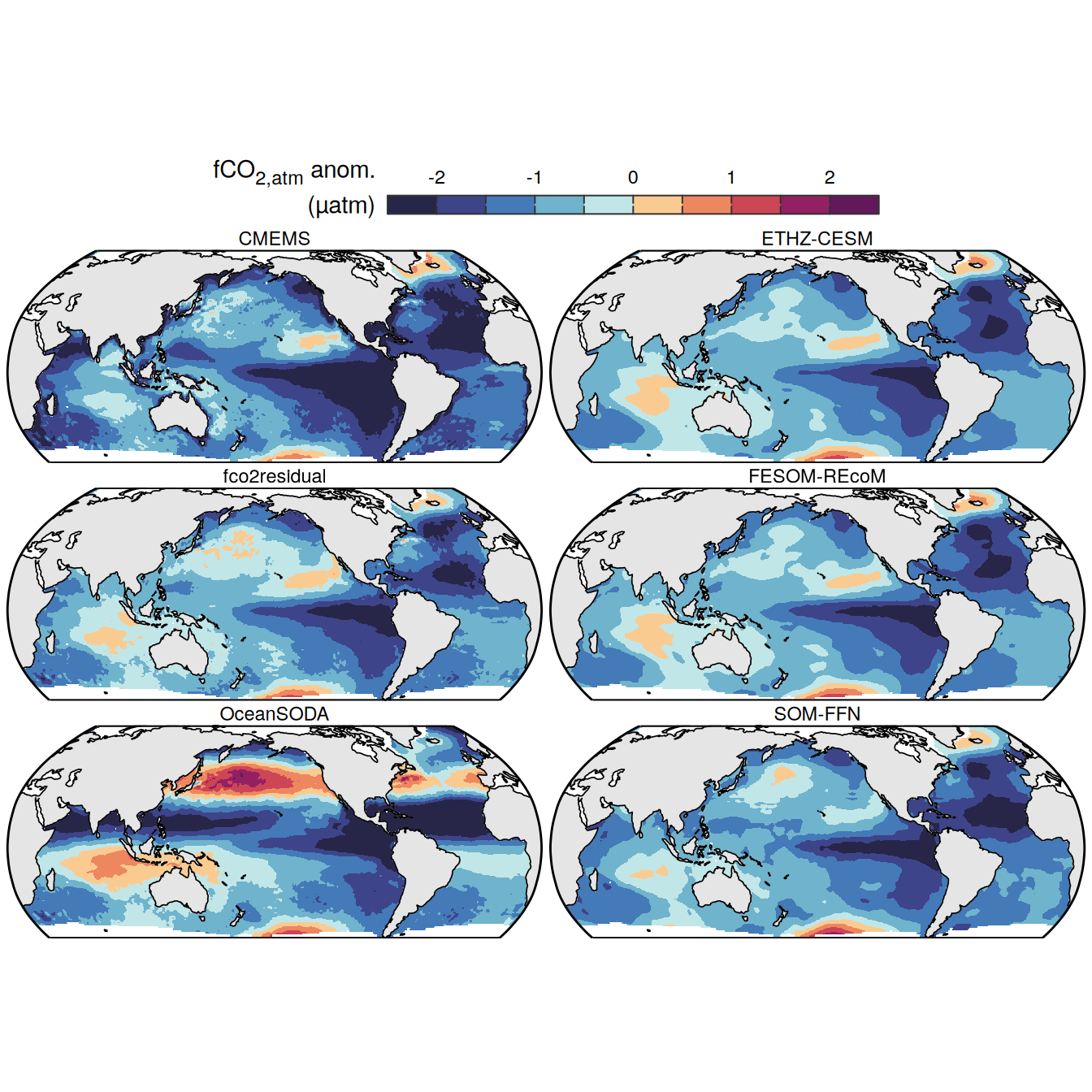
| Version | Author | Date |
|---|---|---|
| 1398df0 | jens-daniel-mueller | 2025-03-14 |
| 17f843d | jens-daniel-mueller | 2025-03-10 |
| fb85a52 | jens-daniel-mueller | 2025-03-10 |
| ae5b6a4 | jens-daniel-mueller | 2025-03-10 |
| b9e8f8c | jens-daniel-mueller | 2025-03-10 |
| 9fe7d3d | jens-daniel-mueller | 2025-03-02 |
| 9276be7 | jens-daniel-mueller | 2025-03-02 |
| 417f35d | jens-daniel-mueller | 2025-02-28 |
| d532d40 | jens-daniel-mueller | 2025-02-28 |
| 518e3d0 | jens-daniel-mueller | 2025-02-27 |
[[4]]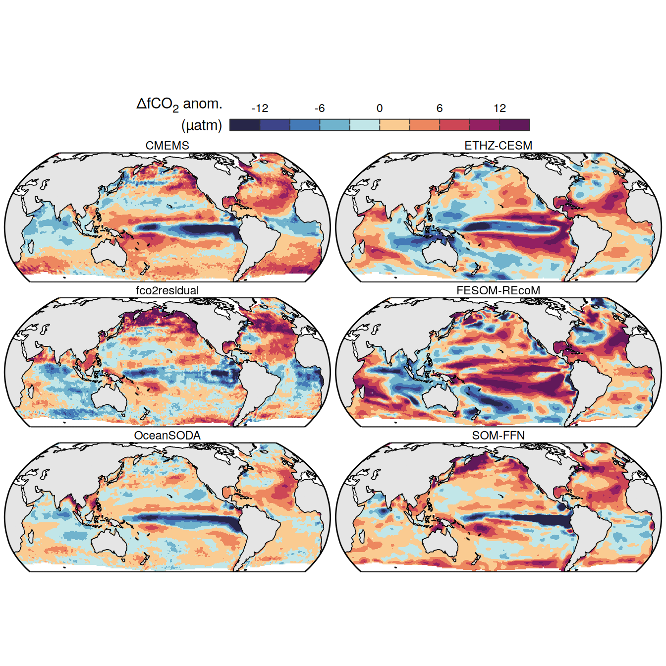
[[5]]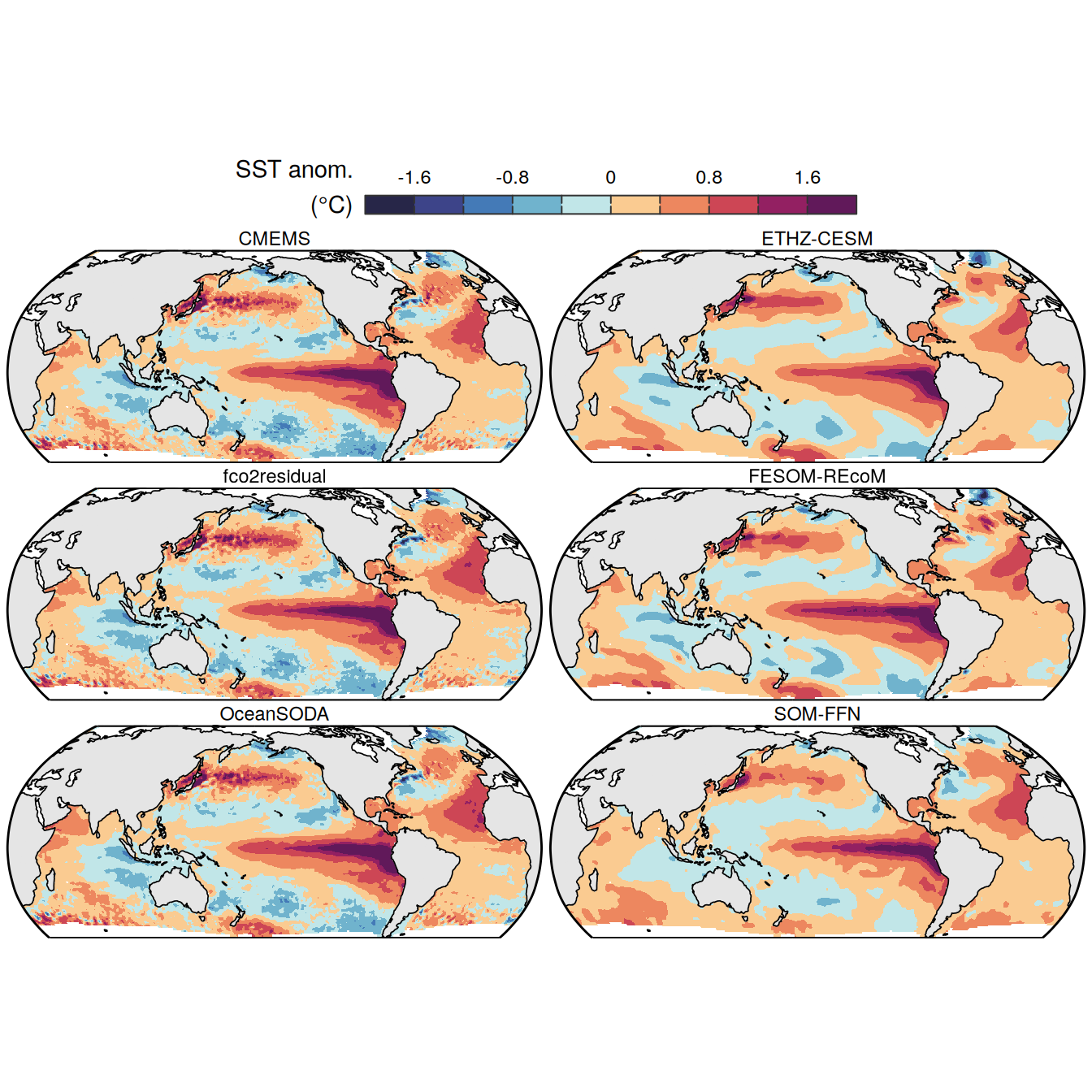
[[6]]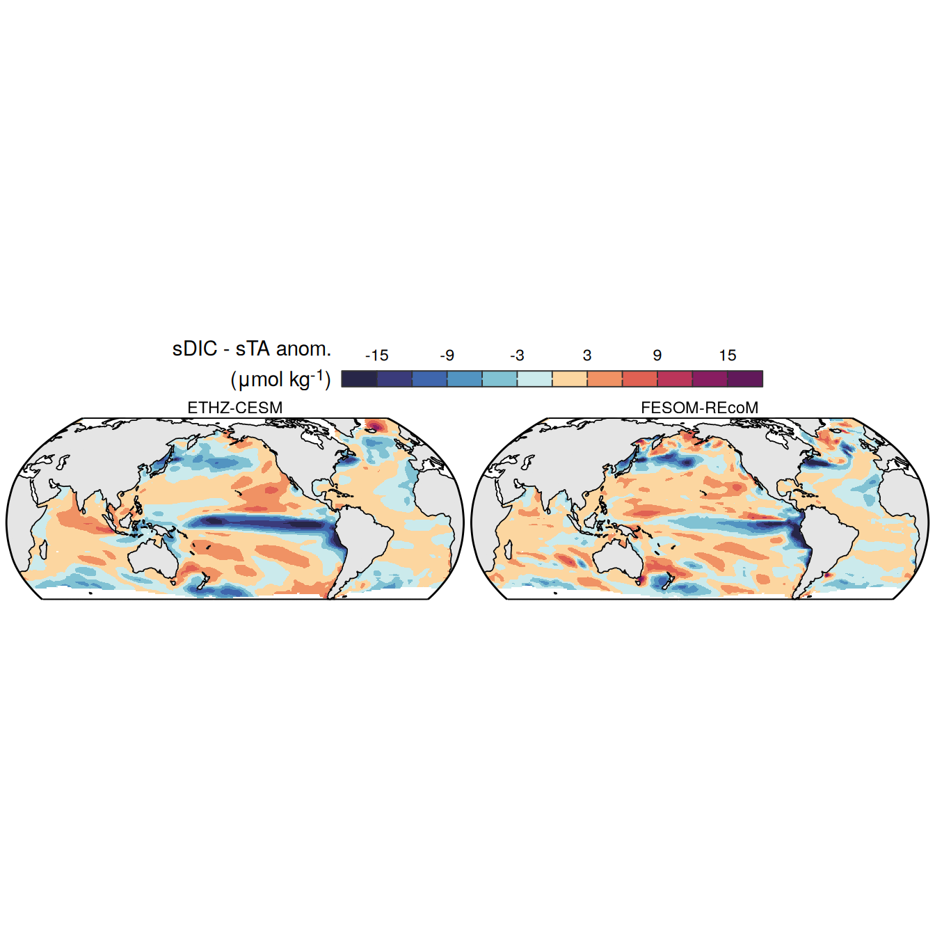
[[7]]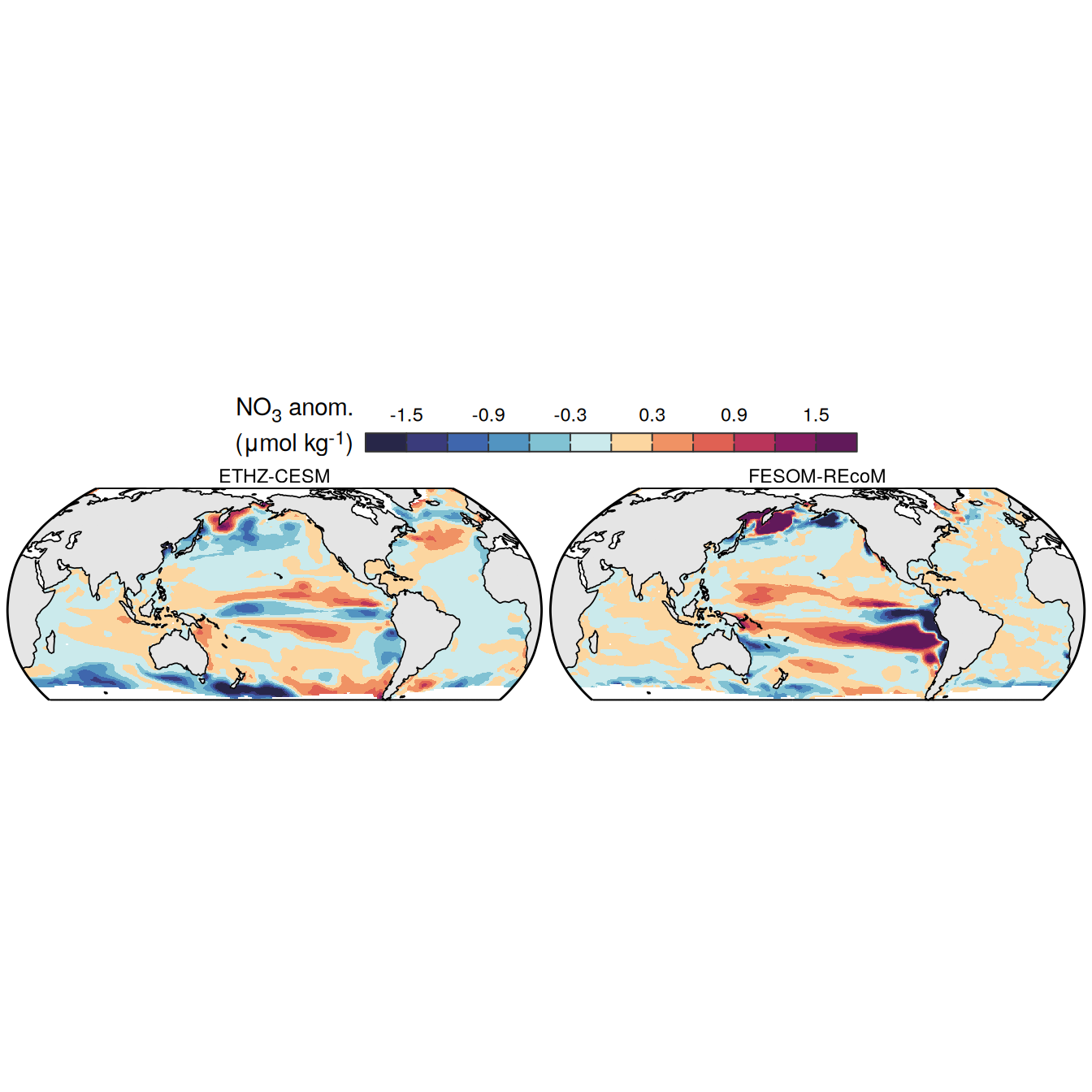
[[8]]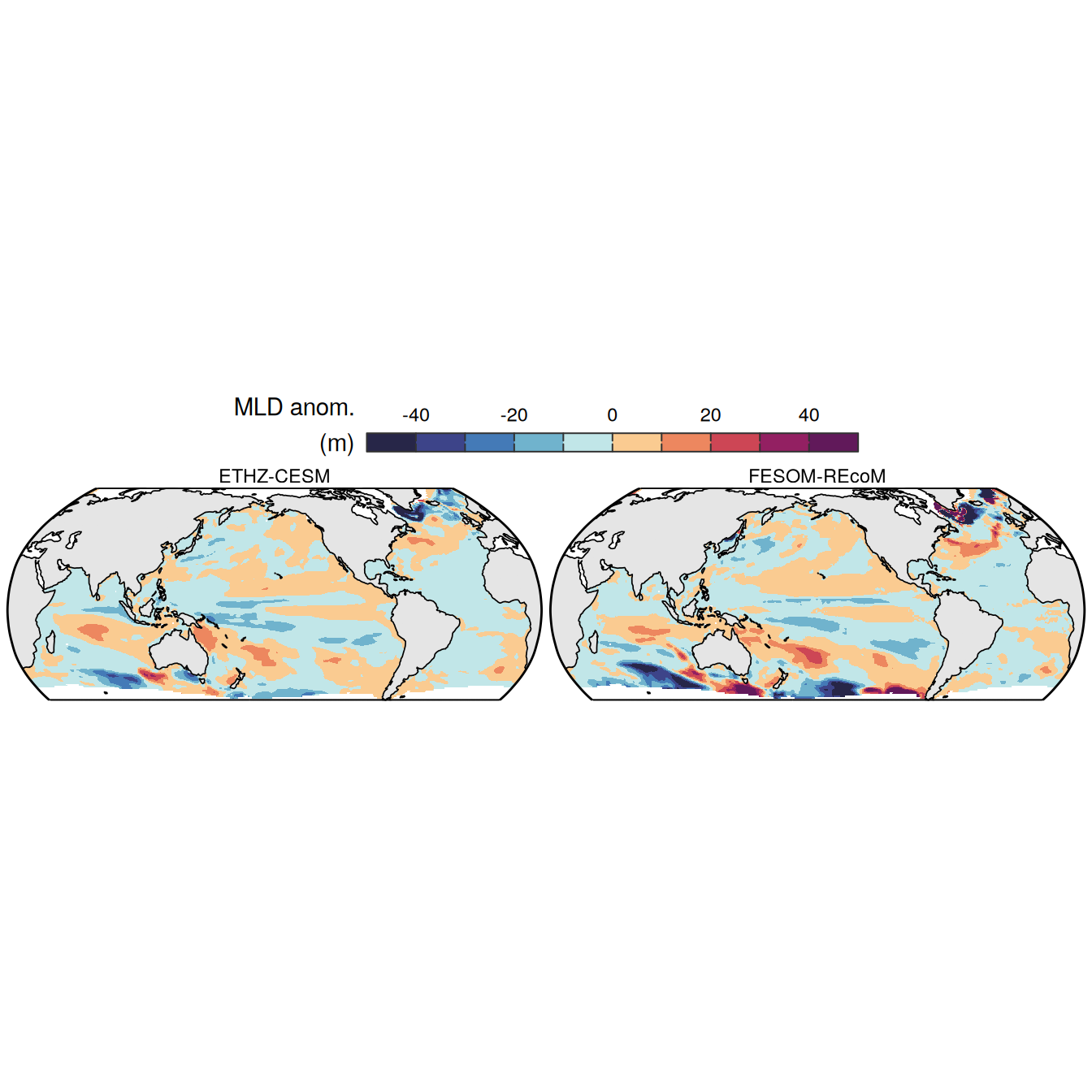
[[9]]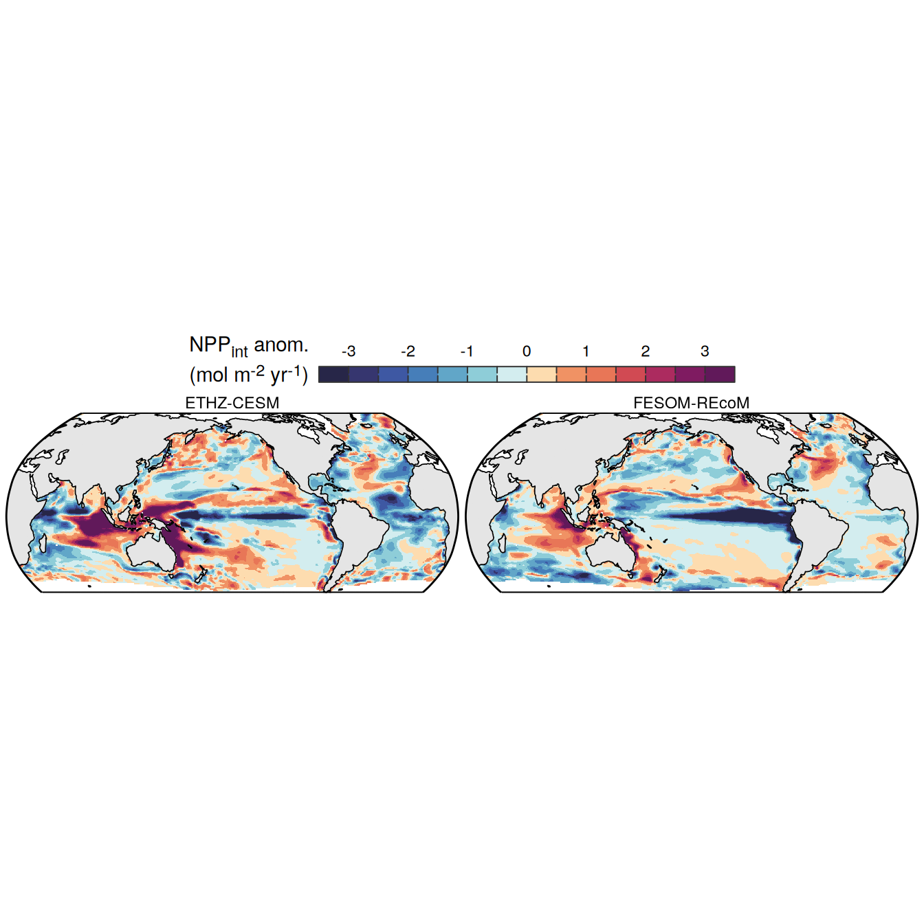
| Version | Author | Date |
|---|---|---|
| 1398df0 | jens-daniel-mueller | 2025-03-14 |
[[10]]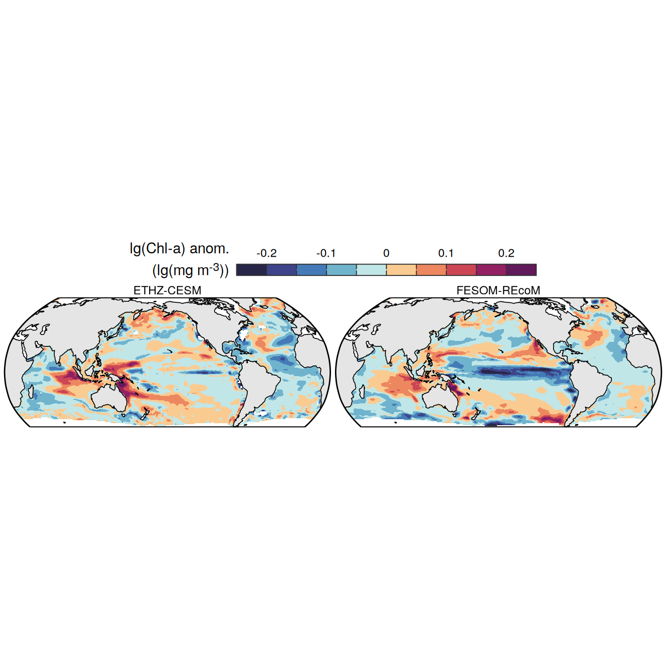
| Version | Author | Date |
|---|---|---|
| 1398df0 | jens-daniel-mueller | 2025-03-14 |
plot_list <-
pco2_product_map_annual_anomaly %>%
  filter(year == 2023,
         product == "ETHZ-CESM",
         name %in% c(
           "fgco2",
           "dfco2",
           "kw_sol",
           "temperature",
           "salinity",
           "sdissic",
           "stalk",
           "sdissic_stalk",
           "no3",
           "mld",
           "intpp",
           "chl"
         )) %>%
  group_split(name) %>%
  # head(1) %>%
  map(
    ~ p_map_mdim_robinson(
      df = .x,
      var = "resid",
      legend_title = labels_breaks(.x %>% distinct(name))$i_legend_title,
      breaks = labels_breaks(.x %>% distinct(name))$i_breaks
    )
  )


ggsave(plot = wrap_plots(plot_list,
                         ncol = 3,
                         byrow = FALSE),
       width = 14,
       height = 11,
       filename = "../output/map_anomaly_ETHZ-CESM.pdf")
plot_list <-
pco2_product_map_annual_anomaly %>%
filter(year == 2023,
product == "FESOM-REcoM",
name %in% c(
"fgco2",
"dfco2",
"kw_sol",
"temperature",
"salinity",
"sdissic",
"stalk",
"sdissic_stalk",
"no3",
"mld",
"intpp",
"chl"
)) %>%
group_split(name) %>%
# head(1) %>%
map(
~ p_map_mdim_robinson(
df = .x,
var = "resid",
legend_title = labels_breaks(.x %>% distinct(name))$i_legend_title,
breaks = labels_breaks(.x %>% distinct(name))$i_breaks
)
)
ggsave(plot = wrap_plots(plot_list,
ncol = 3,
byrow = FALSE),
width = 14,
height = 11,
filename = "../output/map_anomaly_FESOM-REcoM.pdf")
rm(plot_list)pco2_product_map_annual_anomaly_ensemble <-
pco2_product_map_annual_anomaly %>%
filter(year == 2023,
product %in% pco2_product_list) %>%
fgroup_by(name, lon, lat) %>%
fsummarise(
resid_sd = fsd(resid),
resid_mean = fmean(resid),
value_sd = fsd(value),
value_mean = fmean(value),
n = fnobs(resid)
) %>%
filter(n == length(pco2_product_list)) %>%
select(-n)
pco2_product_map_annual_anomaly_ensemble_coarse <-
m_grid_horizontal_coarse(pco2_product_map_annual_anomaly_ensemble) %>%
fgroup_by(name, lon_grid, lat_grid) %>%
fsummarise(
resid_sd_coarse = fmean(resid_sd, na.rm = TRUE),
resid_mean_coarse = fmean(resid_mean, na.rm = TRUE),
value_sd_coarse = fmean(value_sd, na.rm = TRUE),
value_mean_coarse = fmean(value_mean, na.rm = TRUE)
) %>%
rename(lon = lon_grid, lat = lat_grid)
pco2_product_map_annual_anomaly_ensemble_uncertainty <-
pco2_product_map_annual_anomaly_ensemble_coarse %>%
mutate(signif_single = if_else(abs(resid_mean_coarse) < resid_sd_coarse, 0, 1)) %>%
select(lon, lat, name, signif_single) %>%
st_as_sf(coords = c("lon", "lat"), crs = "+proj=longlat")
pco2_product_map_annual_anomaly_ensemble %>%
mutate(product = "Ensemble mean") %>%
group_split(name) %>%
# head(1) %>%
map(
~ p_map_mdim_robinson(
df = .x,
df_uncertainty = pco2_product_map_annual_anomaly_ensemble_uncertainty %>%
filter(name == .x %>% distinct(name) %>% pull()),
var = "resid_mean",
legend_title = labels_breaks(.x %>% distinct(name))$i_legend_title,
breaks = labels_breaks(.x %>% distinct(name))$i_breaks,
n_labels = 2
)
)[[1]]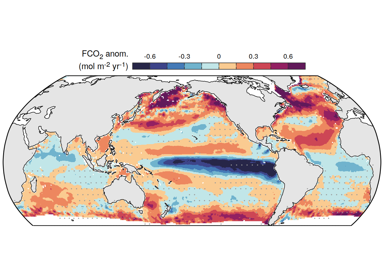
| Version | Author | Date |
|---|---|---|
| 42ecae0 | jens-daniel-mueller | 2025-03-13 |
| 17f843d | jens-daniel-mueller | 2025-03-10 |
| fb85a52 | jens-daniel-mueller | 2025-03-10 |
| ae5b6a4 | jens-daniel-mueller | 2025-03-10 |
| b9e8f8c | jens-daniel-mueller | 2025-03-10 |
| 9fe7d3d | jens-daniel-mueller | 2025-03-02 |
| 417f35d | jens-daniel-mueller | 2025-02-28 |
| d532d40 | jens-daniel-mueller | 2025-02-28 |
| 518e3d0 | jens-daniel-mueller | 2025-02-27 |
[[2]]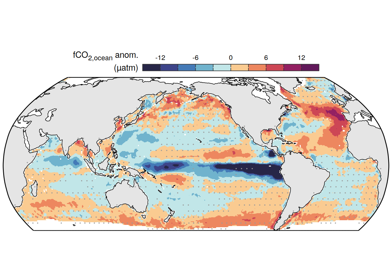
| Version | Author | Date |
|---|---|---|
| 1398df0 | jens-daniel-mueller | 2025-03-14 |
| 17f843d | jens-daniel-mueller | 2025-03-10 |
| fb85a52 | jens-daniel-mueller | 2025-03-10 |
| ae5b6a4 | jens-daniel-mueller | 2025-03-10 |
| b9e8f8c | jens-daniel-mueller | 2025-03-10 |
| 9fe7d3d | jens-daniel-mueller | 2025-03-02 |
| 417f35d | jens-daniel-mueller | 2025-02-28 |
| d532d40 | jens-daniel-mueller | 2025-02-28 |
| 518e3d0 | jens-daniel-mueller | 2025-02-27 |
[[3]]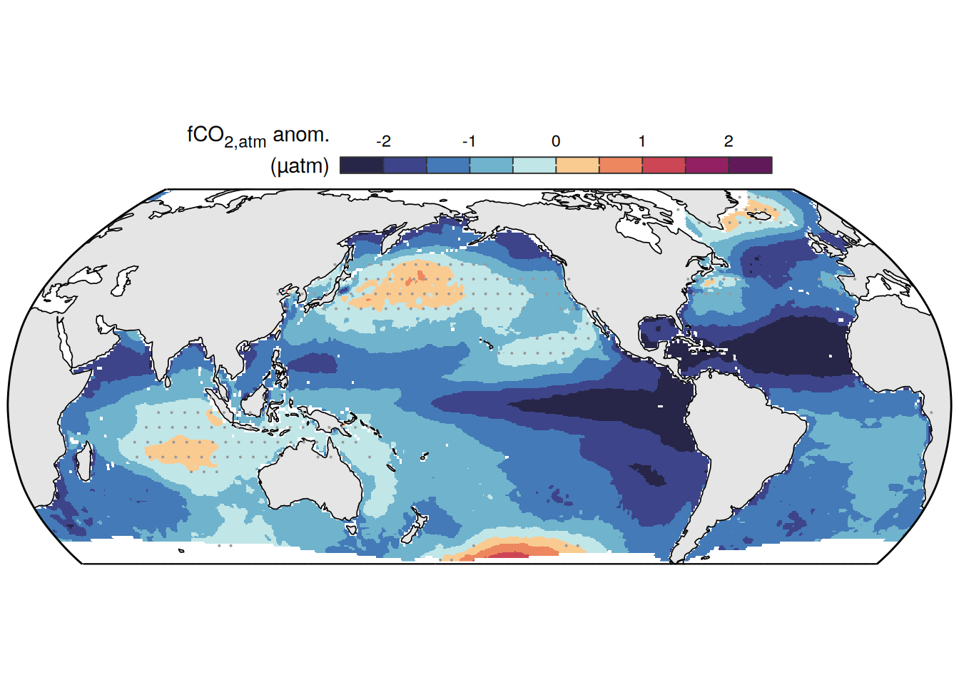
| Version | Author | Date |
|---|---|---|
| 1398df0 | jens-daniel-mueller | 2025-03-14 |
| 17f843d | jens-daniel-mueller | 2025-03-10 |
| fb85a52 | jens-daniel-mueller | 2025-03-10 |
| ae5b6a4 | jens-daniel-mueller | 2025-03-10 |
| b9e8f8c | jens-daniel-mueller | 2025-03-10 |
| 9fe7d3d | jens-daniel-mueller | 2025-03-02 |
| 417f35d | jens-daniel-mueller | 2025-02-28 |
| d532d40 | jens-daniel-mueller | 2025-02-28 |
| 518e3d0 | jens-daniel-mueller | 2025-02-27 |
[[4]]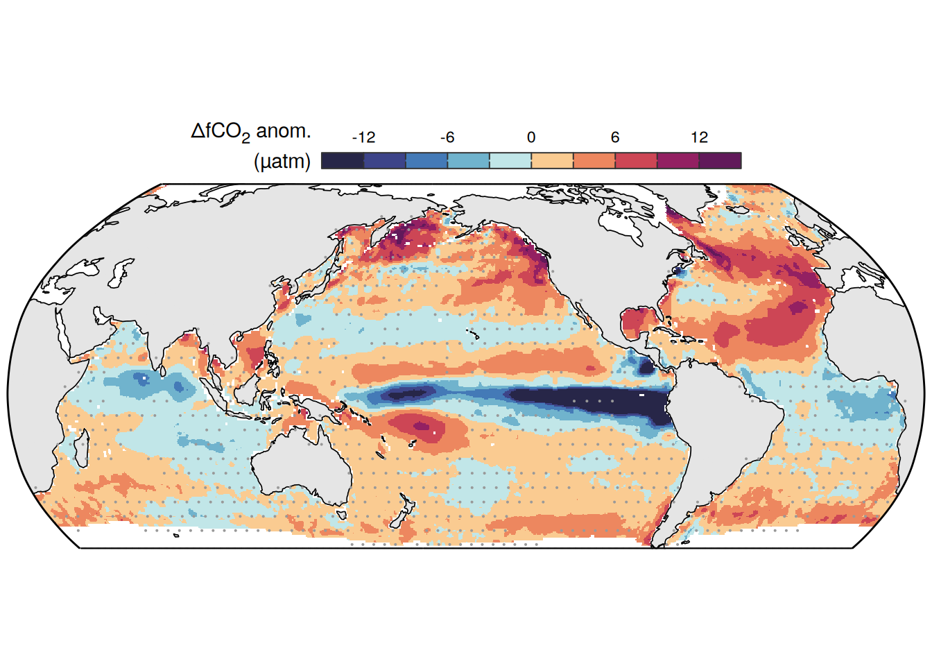
| Version | Author | Date |
|---|---|---|
| 1398df0 | jens-daniel-mueller | 2025-03-14 |
| 17f843d | jens-daniel-mueller | 2025-03-10 |
| fb85a52 | jens-daniel-mueller | 2025-03-10 |
| ae5b6a4 | jens-daniel-mueller | 2025-03-10 |
| b9e8f8c | jens-daniel-mueller | 2025-03-10 |
| 9fe7d3d | jens-daniel-mueller | 2025-03-02 |
| 417f35d | jens-daniel-mueller | 2025-02-28 |
| d532d40 | jens-daniel-mueller | 2025-02-28 |
| 518e3d0 | jens-daniel-mueller | 2025-02-27 |
[[5]]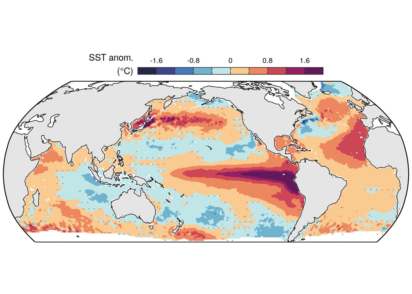
| Version | Author | Date |
|---|---|---|
| 1398df0 | jens-daniel-mueller | 2025-03-14 |
plot_list <- pco2_product_map_annual_anomaly_ensemble %>%
  mutate(product = "Ensemble mean") %>%
  filter(name %in% c("fgco2", "temperature")) %>%
  group_split(name) %>%
  map(
    ~ p_map_mdim_robinson(
      df = .x,
      df_uncertainty = pco2_product_map_annual_anomaly_ensemble_uncertainty %>%
        filter(name == .x %>% distinct(name) %>% pull()),
      var = "resid_mean",
      legend_title = labels_breaks(.x %>% distinct(name))$i_legend_title,
      legend_position = "bottom",
      breaks = labels_breaks(.x %>% distinct(name))$i_breaks,
      n_labels = 2
    )
  )

ggsave(plot = wrap_plots(rev(plot_list),
                         ncol = 2,
                         byrow = TRUE),
       width = 10,
       height = 3,
       dpi = 900,
       filename = "../output/Fig1_cd.pdf")


pco2_product_map_annual_anomaly_ensemble_uncertainty <-
  pco2_product_map_annual_anomaly_ensemble_coarse %>%
  mutate(signif_single = if_else(abs(value_mean_coarse) < value_sd_coarse, 0, 1)) %>%
  select(lon, lat, name, signif_single) %>%
  st_as_sf(coords = c("lon", "lat"), crs = "+proj=longlat")

pco2_product_map_annual_anomaly_ensemble %>%
  mutate(product = "Ensemble mean") %>%
  filter(name %in% c("fgco2")) %>%
  group_split(name) %>%
  map(
    ~ p_map_mdim_robinson(
      df = .x,
      df_uncertainty = pco2_product_map_annual_anomaly_ensemble_uncertainty %>%
        filter(name == .x %>% distinct(name) %>% pull()),
      var = "value_mean",
      legend_title = str_remove(
        labels_breaks(.x %>% distinct(name))$i_legend_title,
        " anom."),
      breaks = c(-Inf, seq(-4,4,1), Inf),
      n_labels = 2
    )
  )
[[1]]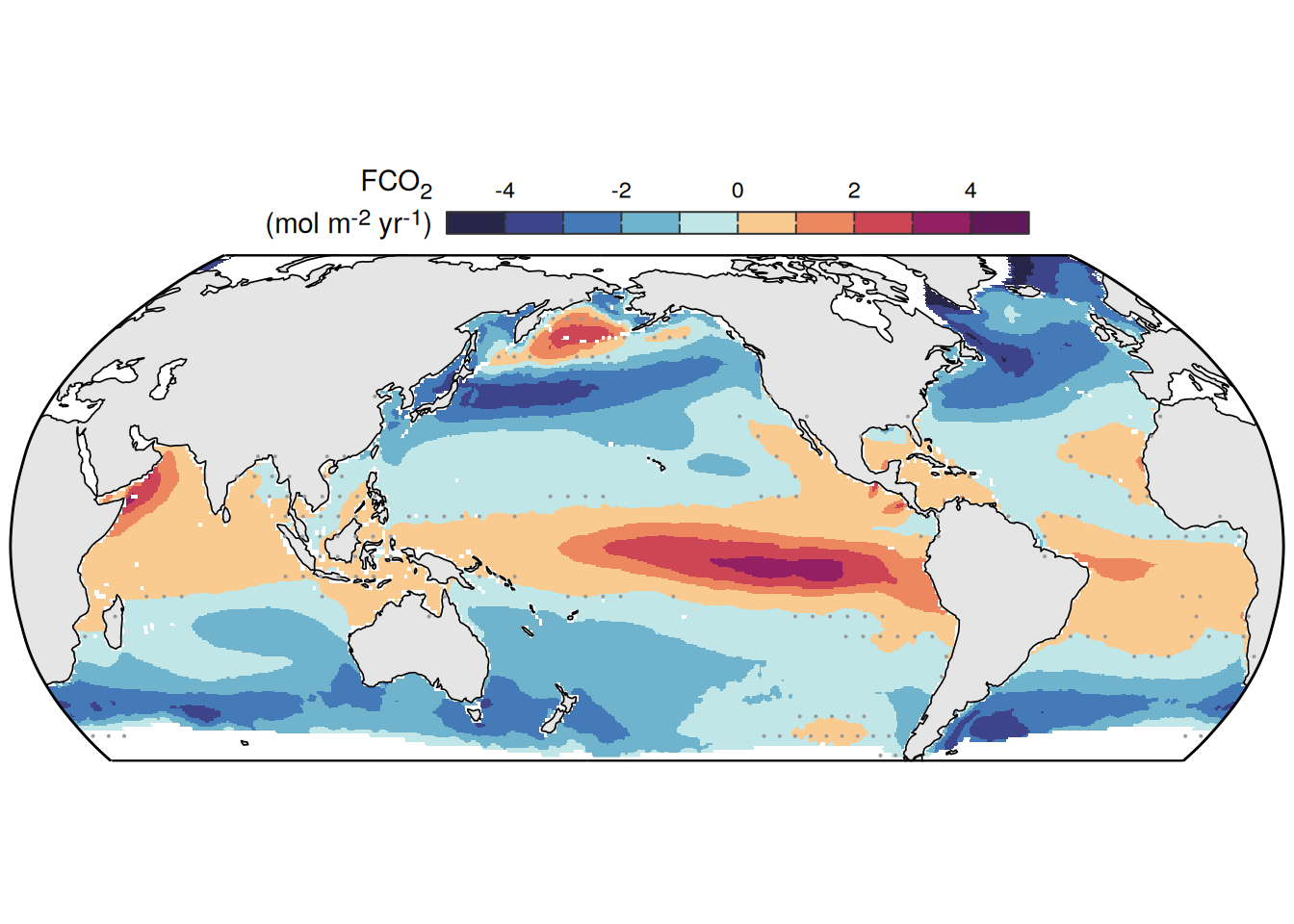
| Version | Author | Date |
|---|---|---|
| 1398df0 | jens-daniel-mueller | 2025-03-14 |
ggsave(width = 5,
       height = 3,
       filename = "../output/map_absolute_ensemble_mean_pco2_products.pdf")


rm(pco2_product_map_annual_anomaly_ensemble_uncertainty)
pco2_product_map_annual_anomaly_ensemble_offset <-
left_join(
pco2_product_map_annual_anomaly_ensemble,
pco2_product_map_annual_anomaly %>%
filter(year == 2023,
product %in% pco2_product_list)
) %>%
mutate(`Anomaly offset` = resid - resid_mean) %>%
select(name, lon, lat, product, `Anomaly offset`)
pco2_product_map_annual_anomaly_ensemble_baseline <-
pco2_product_map_annual_anomaly %>%
filter(year == 2023,
product %in% pco2_product_list) %>%
group_by(name, lon, lat) %>%
summarize(
fit_mean = mean(fit),
n = n()
) %>%
ungroup() %>%
filter(n == length(pco2_product_list)) %>%
select(-n)
pco2_product_map_annual_anomaly_ensemble_baseline <-
left_join(
pco2_product_map_annual_anomaly_ensemble_baseline,
pco2_product_map_annual_anomaly %>%
filter(year == 2023,
product %in% pco2_product_list)
) %>%
mutate(`Baseline offset` = fit - fit_mean) %>%
select(name, lon, lat, product, `Baseline offset`)
full_join(
pco2_product_map_annual_anomaly_ensemble_offset,
pco2_product_map_annual_anomaly_ensemble_baseline
) %>%
pivot_longer(contains("offset"),
names_to = "offset") %>%
group_split(name) %>%
# head(1) %>%
map(
~ map +
geom_tile(data = .x,
aes(lon, lat, fill = value)) +
labs(title = paste(2023, "offset from ensemble mean")) +
scale_fill_gradientn(
colours = warm_cool_gradient,
rescaler = ~ scales::rescale_mid(.x, mid = 0),
name = labels_breaks(.x %>% distinct(name))$i_legend_title,
limits = c(quantile(.x$value, .01), quantile(.x$value, .99)),
oob = squish
) +
facet_grid(product ~ offset) +
guides(
fill = guide_colorbar(
barheight = unit(0.3, "cm"),
barwidth = unit(6, "cm"),
ticks = TRUE,
ticks.colour = "grey20",
frame.colour = "grey20",
label.position = "top",
direction = "horizontal"
)
) +
theme(legend.title = element_markdown(), legend.position = "top")
)
rm(pco2_product_map_annual_anomaly_ensemble_offset,
pco2_product_map_annual_anomaly_ensemble_baseline)
gc()pco2_product_map_annual_anomaly_ensemble_gobm <-
pco2_product_map_annual_anomaly %>%
filter(year == 2023,
product %in% gobm_product_list) %>%
group_by(name, lon, lat) %>%
summarize(
resid_sd = sd(resid),
resid_range = max(resid) - min(resid),
resid_mean = mean(resid),
n = n()
) %>%
ungroup() %>%
filter(n == length(gobm_product_list)) %>%
select(-n)
plot_list <-
pco2_product_map_annual_anomaly_ensemble_gobm %>%
filter(name %in% c(
"fgco2",
"dfco2",
"kw_sol",
"temperature",
"salinity",
"sdissic",
"stalk",
"sdissic_stalk",
"no3",
"mld",
"intpp",
"chl"
)) %>%
group_split(name) %>%
# head(1) %>%
map(
~ p_map_mdim_robinson(
df = .x,
var = "resid_mean",
legend_title = labels_breaks(.x %>% distinct(name))$i_legend_title,
breaks = labels_breaks(.x %>% distinct(name))$i_breaks
)
)
ggsave(plot = wrap_plots(plot_list,
ncol = 2,
byrow = FALSE),
width = 10,
height = 16,
filename = "../output/map_anomaly_ensemble_mean_gobm.pdf")
rm(plot_list,
pco2_product_map_annual_anomaly_ensemble_gobm)
gc() used (Mb) gc trigger (Mb) max used (Mb)
Ncells 3124912 166.9 7041390 376.1 7041390 376.1
Vcells 334853829 2554.8 599853234 4576.6 599832749 4576.4Bivariate anomaly
bivariate_map <-
  pco2_product_map_annual_anomaly %>%
  filter(year == 2023, name %in% c("fgco2", "temperature")) %>%
  select(product, name, lon, lat, resid) %>%
  pivot_wider(names_from = name, values_from = resid) %>%
  drop_na()

dim_set <- 3


bivariate_map <-
  bivariate_map %>%
  mutate(
    temperature = cut(
      temperature,
      breaks = c(
        min(bivariate_map$temperature),
        0,
        0.3,
        max(bivariate_map$temperature)
      ),
      include.lowest = TRUE
    ),
    fgco2 = cut(
      fgco2,
      breaks = c(
        min(bivariate_map$fgco2),
        0,
        0.1,
        max(bivariate_map$fgco2)
      ),
      include.lowest = TRUE
    )
  )


bivariate_map <-
  bi_class(
    bivariate_map,
    x = temperature,
    y = fgco2,
    dim = dim_set,
    style = "quantile"
  )

bi_breaks <-
  bi_class_breaks(
    bivariate_map,
    x = temperature,
    y = fgco2,
    dim = dim_set,
    style = "quantile",
    dig_lab = 1,
    split = TRUE
  )

bivariate_map_raster <-
bivariate_map %>%
    relocate(lon, lat) %>%
    select(lon, lat, product, bi_class) %>%
    mutate(bi_class_numeric = as.character(as.numeric(as.factor(bi_class))))


bivariate_map_raster_values <-
bivariate_map_raster %>%
  distinct(bi_class, bi_class_numeric)

bivariate_map_raster <- rast(
  bivariate_map_raster %>%
    select(-bi_class) %>%
    pivot_wider(names_from = product,
                values_from = bi_class_numeric),
    crs = "+proj=longlat"
)


bivariate_map_raster <- project(bivariate_map_raster, target_crs, method = "near")

bivariate_map_tibble <- bivariate_map_raster %>%
  as.data.frame(xy = TRUE, na.rm = FALSE) %>%
  as_tibble() %>%
  rename(lon = x, lat = y) %>%
  pivot_longer(-c(lon, lat),
               names_to = "product",
               values_to = "bi_class_numeric") %>%
  drop_na()

bivariate_map_tibble <-
  right_join(
    bivariate_map_tibble,
    bivariate_map_raster_values %>%
      mutate(bi_class_numeric = as.numeric(bi_class_numeric))
  )


ggplot() +
  geom_raster(data = bivariate_map_tibble,
            aes(x = lon, y = lat, fill = bi_class)) +
  bi_scale_fill(pal = "DkBlue2", dim = dim_set, flip_axes = TRUE) +
  geom_sf(data = worldmap_trans, fill = "grey90", col = "grey90") +
  geom_sf(data = coastline_trans, linewidth = 0.3) +
  geom_sf(data = bbox_graticules_trans, linewidth = 0.5) +
  coord_sf(
    crs = target_crs,
    ylim = lat_lim,
    xlim = lon_lim,
    expand = FALSE
  ) +
  theme(
    axis.title = element_blank(),
    axis.text = element_blank(),
    axis.ticks = element_blank(),
    panel.border = element_rect(colour = "transparent"),
    strip.background = element_blank(),
    legend.position = "none"
  ) +
  facet_wrap( ~ product, ncol = 2)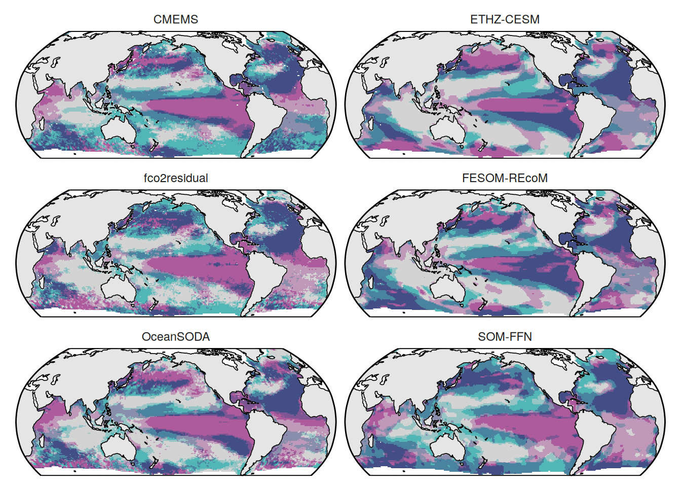
| Version | Author | Date |
|---|---|---|
| 17f843d | jens-daniel-mueller | 2025-03-10 |
| fb85a52 | jens-daniel-mueller | 2025-03-10 |
| ae5b6a4 | jens-daniel-mueller | 2025-03-10 |
| b9e8f8c | jens-daniel-mueller | 2025-03-10 |
| 9fe7d3d | jens-daniel-mueller | 2025-03-02 |
| 417f35d | jens-daniel-mueller | 2025-02-28 |
| d532d40 | jens-daniel-mueller | 2025-02-28 |
| 518e3d0 | jens-daniel-mueller | 2025-02-27 |
ggsave(
width = 6,
height = 5,
dpi = 600,
filename = "../output/map_anomaly_bivariate_all_products.pdf"
)
bi_breaks$bi_x <- bi_breaks$bi_x[-1]
bi_breaks$bi_x[1] <- paste0("-", bi_breaks$bi_x[1])
bi_breaks$bi_y <- bi_breaks$bi_y[-1]
bi_breaks$bi_y[1] <- paste0("-", bi_breaks$bi_y[1])
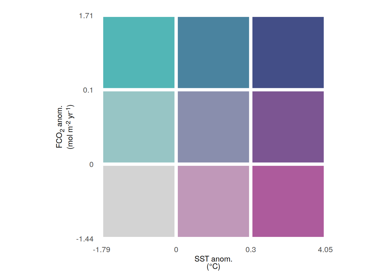
bi_legend(
pal = "DkBlue2",
xlab = labels_breaks("temperature")$i_legend_title,
ylab = labels_breaks("fgco2")$i_legend_title,
dim = dim_set,
pad_width = 2,
breaks = bi_breaks,
arrows = FALSE,
flip_axes = TRUE
) +
theme(
axis.title.x = element_markdown(),
axis.title.y = element_markdown(),
axis.ticks = element_blank(),
axis.text = element_text(size = 10)
)
ggsave(
width = 4,
height = 3,
dpi = 600,
filename = "../output/map_anomaly_bivariate_all_products_legend.pdf"
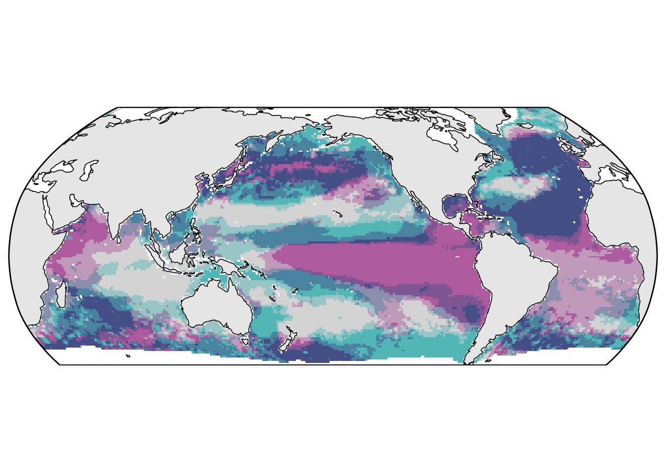
)bivariate_map <-
pco2_product_map_annual_anomaly_ensemble %>%
filter(name %in% c("fgco2", "temperature")) %>%
select(name, lon, lat, resid_mean) %>%
pivot_wider(names_from = name,
values_from = resid_mean) %>%
drop_na()
dim_set <- 3
bivariate_map <-
bivariate_map %>%
mutate(
temperature = cut(
temperature,
breaks = c(
min(bivariate_map$temperature),
0,
0.3,
max(bivariate_map$temperature)
),
include.lowest = TRUE
),
fgco2 = cut(
fgco2,
breaks = c(
max(bivariate_map$fgco2),
0.1,
0,
min(bivariate_map$fgco2)
),
include.lowest = TRUE
)
)
bivariate_map <-
bi_class(
bivariate_map,
x = temperature,
y = fgco2,
dim = dim_set,
style = "quantile"
)
bi_breaks <-
bi_class_breaks(
bivariate_map,
x = temperature,
y = fgco2,
dim = dim_set,
style = "quantile",
dig_lab = 1,
split = TRUE
)
bivariate_map_raster <-
bivariate_map %>%
relocate(lon, lat) %>%
select(lon, lat, bi_class) %>%
mutate(bi_class_numeric = as.character(as.numeric(as.factor(bi_class))))
bivariate_map_raster_values <-
bivariate_map_raster %>%
distinct(bi_class, bi_class_numeric)
bivariate_map_raster <- rast(
bivariate_map_raster %>%
select(-bi_class),
crs = "+proj=longlat"
)
bivariate_map_raster <- project(bivariate_map_raster, target_crs, method = "near")
bivariate_map_tibble <- bivariate_map_raster %>%
as.data.frame(xy = TRUE, na.rm = FALSE) %>%
as_tibble() %>%
rename(lon = x, lat = y) %>%
drop_na()
bivariate_map_tibble <-
right_join(
bivariate_map_tibble,
bivariate_map_raster_values %>%
mutate(bi_class_numeric = as.numeric(bi_class_numeric))
)
ggplot() +
geom_raster(data = bivariate_map_tibble,
aes(x = lon, y = lat, fill = bi_class)) +
bi_scale_fill(pal = "DkBlue2", dim = dim_set, flip_axes = TRUE) +
geom_sf(data = worldmap_trans, fill = "grey90", col = "grey90") +
geom_sf(data = coastline_trans, linewidth = 0.3) +
geom_sf(data = bbox_graticules_trans, linewidth = 0.5) +
coord_sf(
crs = target_crs,
ylim = lat_lim,
xlim = lon_lim,
expand = FALSE
) +
theme(
axis.title = element_blank(),
axis.text = element_blank(),
axis.ticks = element_blank(),
panel.border = element_rect(colour = "transparent"),
strip.background = element_blank(),
legend.position = "none"
)
| Version | Author | Date |
|---|---|---|
| 17f843d | jens-daniel-mueller | 2025-03-10 |
| fb85a52 | jens-daniel-mueller | 2025-03-10 |
| ae5b6a4 | jens-daniel-mueller | 2025-03-10 |
| b9e8f8c | jens-daniel-mueller | 2025-03-10 |
| 9fe7d3d | jens-daniel-mueller | 2025-03-02 |
| 417f35d | jens-daniel-mueller | 2025-02-28 |
| d532d40 | jens-daniel-mueller | 2025-02-28 |
| 518e3d0 | jens-daniel-mueller | 2025-02-27 |
ggsave(width = 5,
       height = 2.5,
       dpi = 1200,
       filename = "../output/Fig5_a_map.pdf")

bi_breaks$bi_x <- bi_breaks$bi_x[-1]
bi_breaks$bi_x[1] <- paste0("-", bi_breaks$bi_x[1])

bi_breaks$bi_y <- bi_breaks$bi_y[-1]
bi_breaks$bi_y[1] <- paste0("-", bi_breaks$bi_y[1])


bi_legend(
  pal = "DkBlue2",
  xlab = labels_breaks("temperature")$i_legend_title,
  ylab = labels_breaks("fgco2")$i_legend_title,
  dim = dim_set,
  pad_width = 2,
  breaks = bi_breaks,
  arrows = FALSE,
  flip_axes = TRUE
) +
  theme(
    axis.title.x = element_markdown(),
    axis.title.y = element_markdown(),
    axis.ticks = element_blank(),
    axis.text = element_text(size = 10)
  )
ggsave(width = 4,
       height = 3,
       dpi = 600,
       filename = "../output/Fig5_a_legend.pdf")
pco2_product_zonal_annual_anomaly <-
pco2_product_hovmoeller_monthly_anomaly %>%
filter(year == 2023) %>%
group_by(product, name, lat) %>%
summarise(resid = mean(resid)) %>%
ungroup()
pco2_product_zonal_annual_anomaly %>%
ggplot(aes(resid, lat, col = product)) +
geom_vline(xintercept = 0) +
geom_hline(yintercept = 0) +
geom_path() +
scale_color_manual(values = color_products) +
facet_wrap( ~ name, scales = "free_x", ncol = 4)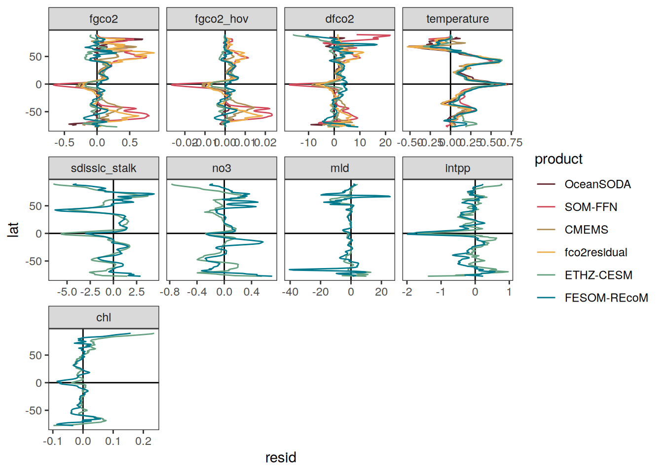
pco2_product_zonal_annual_anomaly_ensemble <-
pco2_product_zonal_annual_anomaly %>%
filter(product %in% pco2_product_list) %>%
group_by(lat, name) %>%
fsummarise(
resid_sd = fsd(resid),
resid_mean = fmean(resid)
)
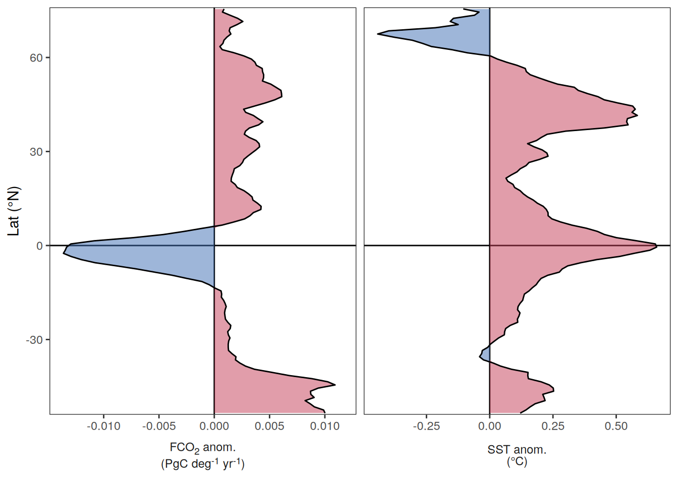
pco2_product_zonal_annual_anomaly_ensemble %>%
filter(name %in% c("fgco2_hov", "temperature")) %>%
ggplot(aes(resid_mean, lat)) +
geom_vline(xintercept = 0) +
geom_hline(yintercept = 0) +
# geom_ribbon(aes(xmin = resid_mean - resid_sd, xmax = resid_mean + resid_sd),
# alpha = 0.5) +
geom_ribbon(aes(xmin = 0, xmax = pmax(0, resid_mean), fill = "Positive"),
alpha = 0.5) +
geom_ribbon(aes(xmax = 0, xmin = pmin(0, resid_mean), fill = "Negative"),
alpha = 0.5) +
scale_fill_manual(values = c(cold_color, warm_color)) +
geom_path() +
facet_grid(. ~ name,
labeller = labeller(name = x_axis_labels),
scales = "free_x",
switch = "x") +
scale_y_continuous(breaks = seq(-60,60,30),
name = "Lat (°N)",
limits = c(-54,76),
expand = c(0,0)) +
theme(
strip.text.x.bottom = element_markdown(),
strip.placement = "outside",
strip.background.x = element_blank(),
axis.title.x = element_blank(),
legend.position = "none"
)
bi_pal("DkBlue2", preview = FALSE) 1-1 2-1 3-1 1-2 2-2 3-2 1-3 2-3
"#d3d3d3" "#97c5c5" "#52b6b6" "#c098b9" "#898ead" "#4a839f" "#ad5b9c" "#7c5592"
3-3
"#434e87" # "#d3d3d3" "#97c5c5" "#52b6b6" "#c098b9" "#898ead" "#4a839f" "#ad5b9c" "#7c5592" "#434e87"
p_zonal_fgco2 <-
pco2_product_zonal_annual_anomaly_ensemble %>%
filter(name %in% c("fgco2_hov")) %>%
mutate(resid_mean = resid_mean * 1000) %>%
ggplot(aes(resid_mean, lat)) +
geom_vline(xintercept = 0) +
geom_ribbon(aes(xmin = 0, xmax = pmax(0, resid_mean), fill = "Positive"),
alpha = 0.9) +
geom_ribbon(aes(xmax = 0, xmin = pmin(0, resid_mean), fill = "Negative"),
alpha = 0.9) +
scale_fill_manual(values = c("#d3d3d3", "#52b6b6")) +
geom_path() +
scale_y_continuous(breaks = seq(-60,60,30),
name = "Lat (°N)",
limits = c(-54,76),
expand = c(0,0)) +
scale_x_continuous(breaks = seq(-5,5,5),
name = str_replace(
labels_breaks("fgco2_hov")$i_legend_title,
"PgC", "TgC"
)) +
theme_classic() +
theme(
legend.position = "none",
axis.title.x = element_markdown(),
axis.text.y = element_blank(),
axis.ticks.y = element_blank(),
axis.title.y = element_blank(),
axis.line.y = element_blank()
)
p_zonal_temperature <-
pco2_product_zonal_annual_anomaly_ensemble %>%
filter(name %in% c("temperature")) %>%
ggplot(aes(resid_mean, lat)) +
geom_vline(xintercept = 0) +
geom_ribbon(aes(xmin = 0, xmax = pmax(0, resid_mean), fill = "Positive"),
alpha = 0.9) +
geom_ribbon(aes(xmax = 0, xmin = pmin(0, resid_mean), fill = "Negative"),
alpha = 0.9) +
scale_fill_manual(values = c("#d3d3d3", "#ad5b9c")) +
geom_path() +
scale_y_continuous(breaks = seq(-60,60,30),
name = "Lat (°N)",
limits = c(-54,76),
expand = c(0,0)) +
scale_x_continuous(breaks = seq(-0.6,0.6,0.3),
name = labels_breaks("temperature")$i_legend_title) +
theme_classic() +
theme(
legend.position = "none",
axis.title.x = element_markdown(),
axis.title.y = element_text(angle = 0)
)
p_zonal_temperature | p_zonal_fgco2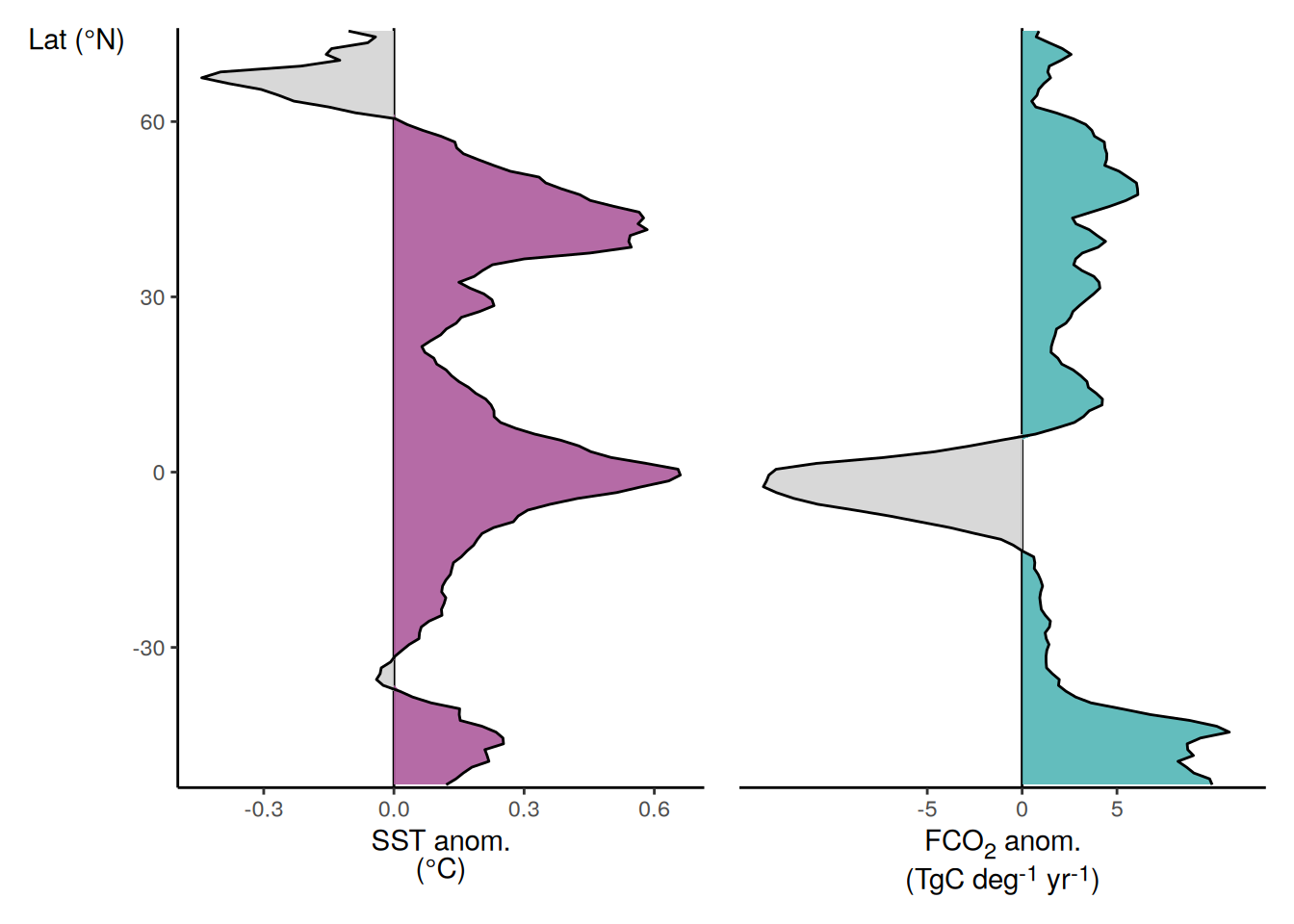
ggsave(width = 2.8,
       height = 4.5,
       filename = "../output/Fig5_b.pdf")

p_zonal_fgco2 <-
pco2_product_zonal_annual_anomaly_ensemble %>%
  filter(name %in% c("fgco2_hov")) %>%
  mutate(resid_mean = resid_mean * 1000) %>%
  ggplot(aes(resid_mean, lat)) +
  geom_vline(xintercept = 0) +
  geom_ribbon(aes(xmin = 0, xmax = pmax(0, resid_mean), fill = "Positive"),
              alpha = 0.9) +
  geom_ribbon(aes(xmax = 0, xmin = pmin(0, resid_mean), fill = "Negative"),
              alpha = 0.9) +
  scale_fill_manual(values = c(cold_color, warm_color)) +
  geom_path() +
  scale_y_continuous(breaks = seq(-60,60,30),
                     name = "Lat (°N)",
                     limits = c(-54,76),
                     expand = c(0,0)) +
  scale_x_continuous(breaks = seq(-5,5,5),
                     name = str_replace(
                       labels_breaks("fgco2_hov")$i_legend_title,
                     "PgC", "TgC"
                     ),
                     position = "top") +
  theme_classic() +
  theme(
    legend.position = "none",
    axis.title.x = element_markdown(),
    axis.text.y = element_blank(),
    axis.ticks.y = element_blank(),
    axis.title.y = element_blank(),
    axis.line.y = element_blank()
  )


p_zonal_temperature <-
pco2_product_zonal_annual_anomaly_ensemble %>%
  filter(name %in% c("temperature")) %>%
  ggplot(aes(resid_mean, lat)) +
  geom_vline(xintercept = 0) +
  geom_ribbon(aes(xmin = 0, xmax = pmax(0, resid_mean), fill = "Positive"),
              alpha = 0.9) +
  geom_ribbon(aes(xmax = 0, xmin = pmin(0, resid_mean), fill = "Negative"),
              alpha = 0.9) +
  scale_fill_manual(values = c(cold_color, warm_color)) +
  geom_path() +
  scale_y_continuous(breaks = seq(-60,60,30),
                     name = "Lat (°N)",
                     limits = c(-54,76),
                     expand = c(0,0)) +
  scale_x_continuous(breaks = seq(-0.5,0.5,0.5),
                     name = labels_breaks("temperature")$i_legend_title,
                     position = "top") +
  theme_classic() +
  theme(
    legend.position = "none",
    axis.title.x = element_markdown(),
    axis.text.y = element_blank(),
    axis.ticks.y = element_blank(),
    axis.title.y = element_blank(),
    axis.line.y = element_blank()
  )

p_zonal_temperature | p_zonal_fgco2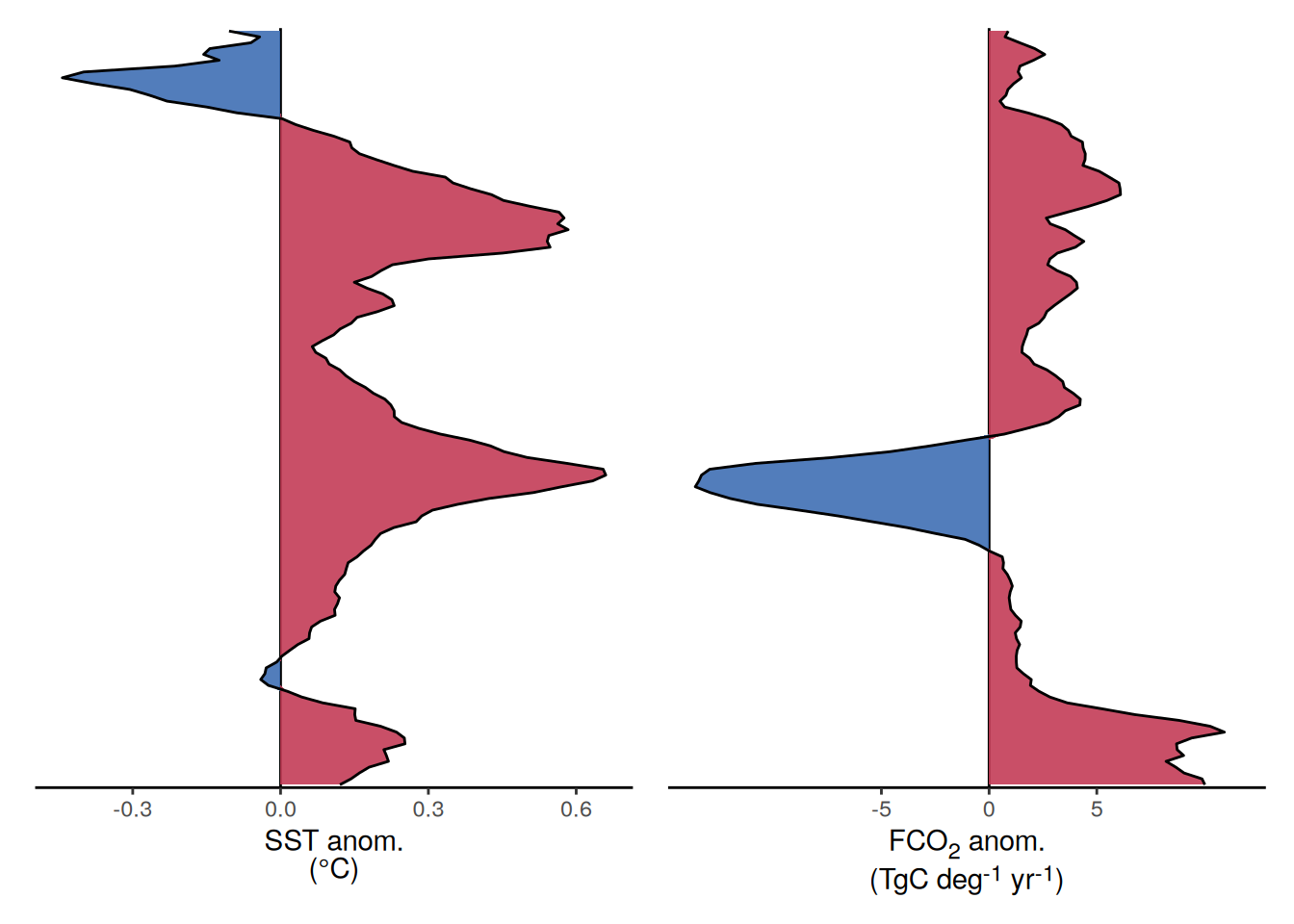
ggsave(width = 2.2,
       height = 3.5,
       dpi = 900,
       filename = "../output/zonal_mean_anomaly_pco2_product_ensemble_mean_warm_cold_color.pdf")
SST flux slope
pco2_product_map_annual_anomaly_temperature_predict <-
pco2_product_map_annual_anomaly_temperature_predict %>%
drop_na()
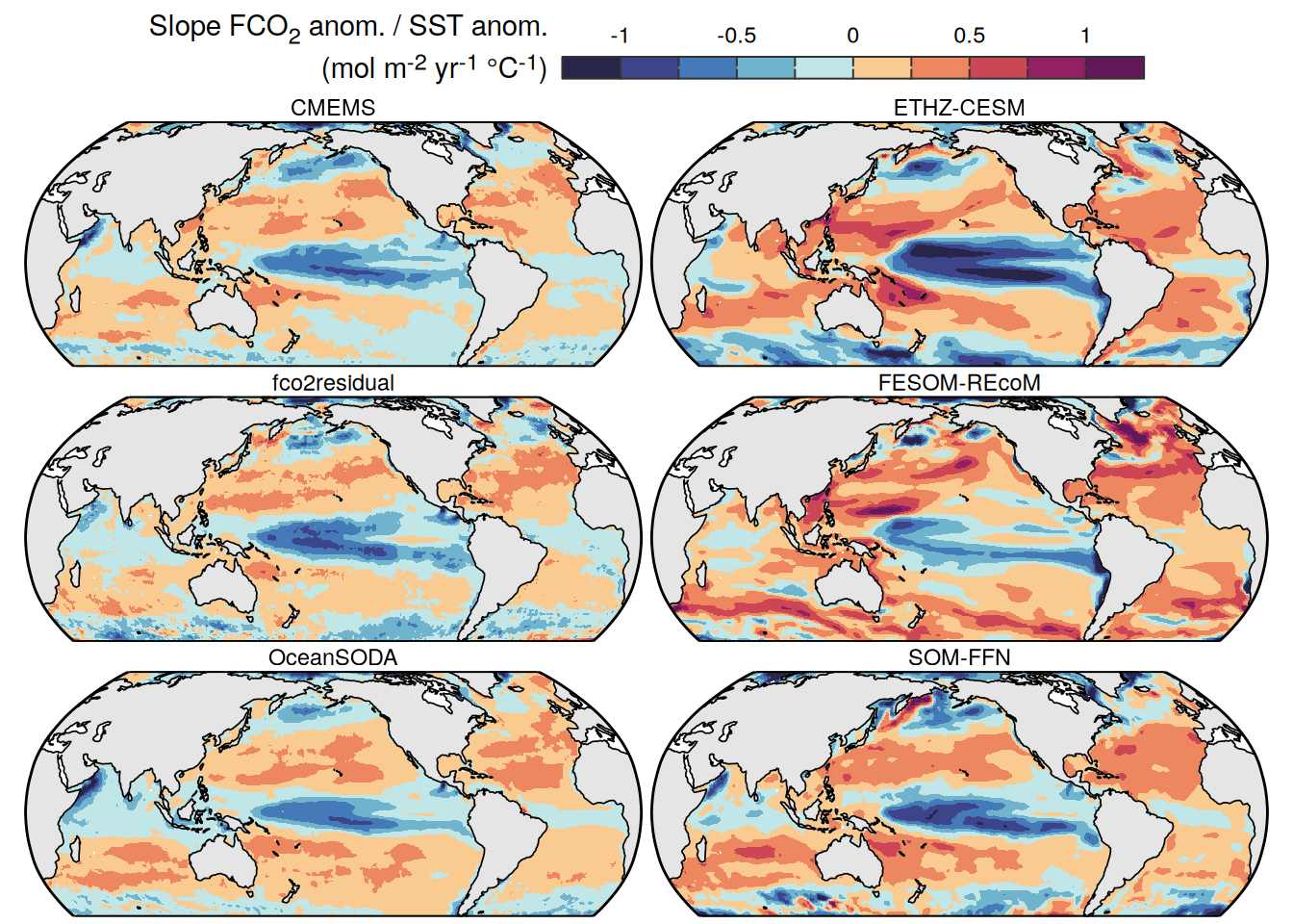
pco2_product_map_annual_anomaly_temperature_predict %>%
p_map_mdim_robinson(
var = "slope",
legend_title = "Slope FCO<sub>2</sub> anom. / SST anom.<br>(mol m<sup>-2</sup> yr<sup>-1</sup> °C<sup>-1</sup>)",
breaks = c(-Inf, seq(-1, 1, 0.25), Inf),
dim_wrap = "product",
n_col = 2
)
ggsave(width = 7,
       height = 6,
       dpi = 600,
       filename = "../output/map_anomaly_correlation_all_products.pdf")


pco2_product_map_annual_anomaly_temperature_predict <-
  pco2_product_map_annual_anomaly_temperature_predict %>%
  select(-year) %>%
  pivot_longer(-c(product, lon, lat), values_to = "resid")


pco2_product_map_annual_anomaly_temperature_predict %>%
  filter(str_detect(name, "fgco2")) %>%
  p_map_mdim_robinson(
    var = "resid",
    legend_title = labels_breaks("fgco2")$i_legend_title,
    breaks = labels_breaks("fgco2")$i_breaks,
    dim_row = "product",
    dim_col = "name"
  )
| Version | Author | Date |
|---|---|---|
| 42ecae0 | jens-daniel-mueller | 2025-03-13 |
| 17f843d | jens-daniel-mueller | 2025-03-10 |
| ae5b6a4 | jens-daniel-mueller | 2025-03-10 |
| b9e8f8c | jens-daniel-mueller | 2025-03-10 |
| 9fe7d3d | jens-daniel-mueller | 2025-03-02 |
| 417f35d | jens-daniel-mueller | 2025-02-28 |
| d532d40 | jens-daniel-mueller | 2025-02-28 |
| 518e3d0 | jens-daniel-mueller | 2025-02-27 |
pco2_product_map_annual_anomaly_temperature_predict_ensemble <-
  pco2_product_map_annual_anomaly_temperature_predict %>%
  filter(product %in% pco2_product_list) %>%
  fgroup_by(name, lon, lat) %>%
  fsummarise(
    resid_sd = fsd(resid),
    resid_mean = fmean(resid),
    n = fnobs(resid)
  ) %>%
  filter(n == length(pco2_product_list)) %>%
  select(-n)


pco2_product_map_annual_anomaly_temperature_predict_ensemble_coarse <-
  m_grid_horizontal_coarse(pco2_product_map_annual_anomaly_temperature_predict_ensemble) %>%
  fgroup_by(name, lon_grid, lat_grid) %>%
  fsummarise(
    resid_sd_coarse = fmean(resid_sd, na.rm = TRUE),
    resid_mean_coarse = fmean(resid_mean, na.rm = TRUE)
  ) %>%
  rename(lon = lon_grid, lat = lat_grid)

pco2_product_map_annual_anomaly_temperature_predict_ensemble_uncertainty <-
  pco2_product_map_annual_anomaly_temperature_predict_ensemble_coarse %>%
  mutate(signif_single = if_else(abs(resid_mean_coarse) < resid_sd_coarse, 0, 1)) %>%
  select(lon, lat, name, signif_single) %>%
  st_as_sf(coords = c("lon", "lat"), crs = "+proj=longlat")


pco2_product_map_annual_anomaly_temperature_predict_ensemble %>%
  mutate(product = "Ensemble mean") %>%
  group_split(name) %>%
  # head(1) %>%
  map(
    ~ p_map_mdim_robinson(
      df = .x,
      df_uncertainty = pco2_product_map_annual_anomaly_temperature_predict_ensemble_uncertainty %>%
        filter(name == .x %>% distinct(name) %>% pull()),
      var = "resid_mean",
      legend_title = labels_breaks(.x %>% distinct(name))$i_legend_title,
      breaks = labels_breaks(.x %>% distinct(name))$i_breaks,
      n_labels = 2
    )
  )
[[1]]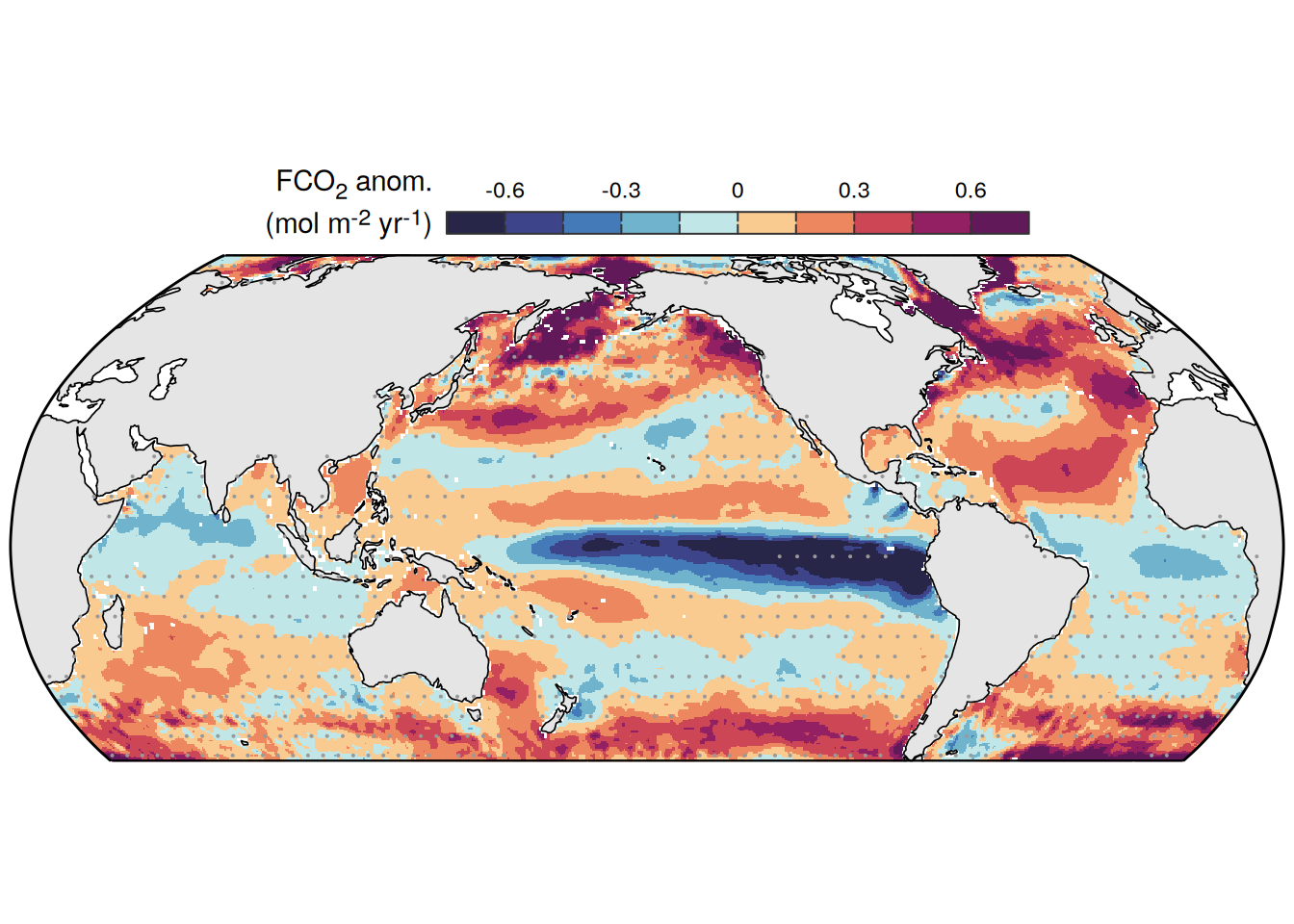
| Version | Author | Date |
|---|---|---|
| 42ecae0 | jens-daniel-mueller | 2025-03-13 |
| 17f843d | jens-daniel-mueller | 2025-03-10 |
| ae5b6a4 | jens-daniel-mueller | 2025-03-10 |
| b9e8f8c | jens-daniel-mueller | 2025-03-10 |
| 9fe7d3d | jens-daniel-mueller | 2025-03-02 |
| 417f35d | jens-daniel-mueller | 2025-02-28 |
| d532d40 | jens-daniel-mueller | 2025-02-28 |
| 518e3d0 | jens-daniel-mueller | 2025-02-27 |
[[2]]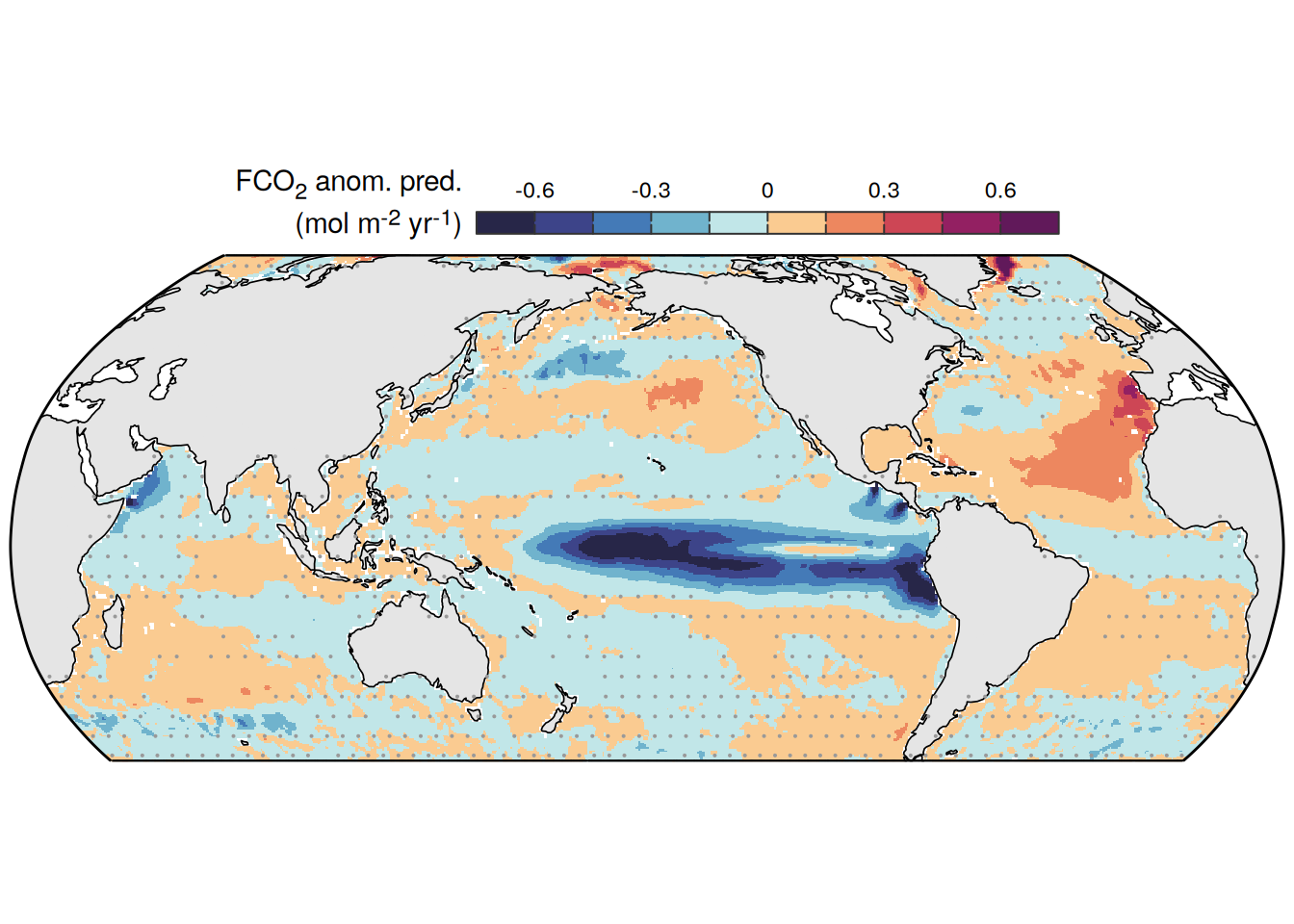
| Version | Author | Date |
|---|---|---|
| 42ecae0 | jens-daniel-mueller | 2025-03-13 |
| 17f843d | jens-daniel-mueller | 2025-03-10 |
| ae5b6a4 | jens-daniel-mueller | 2025-03-10 |
| b9e8f8c | jens-daniel-mueller | 2025-03-10 |
| 9fe7d3d | jens-daniel-mueller | 2025-03-02 |
| 417f35d | jens-daniel-mueller | 2025-02-28 |
| d532d40 | jens-daniel-mueller | 2025-02-28 |
| 518e3d0 | jens-daniel-mueller | 2025-02-27 |
[[3]]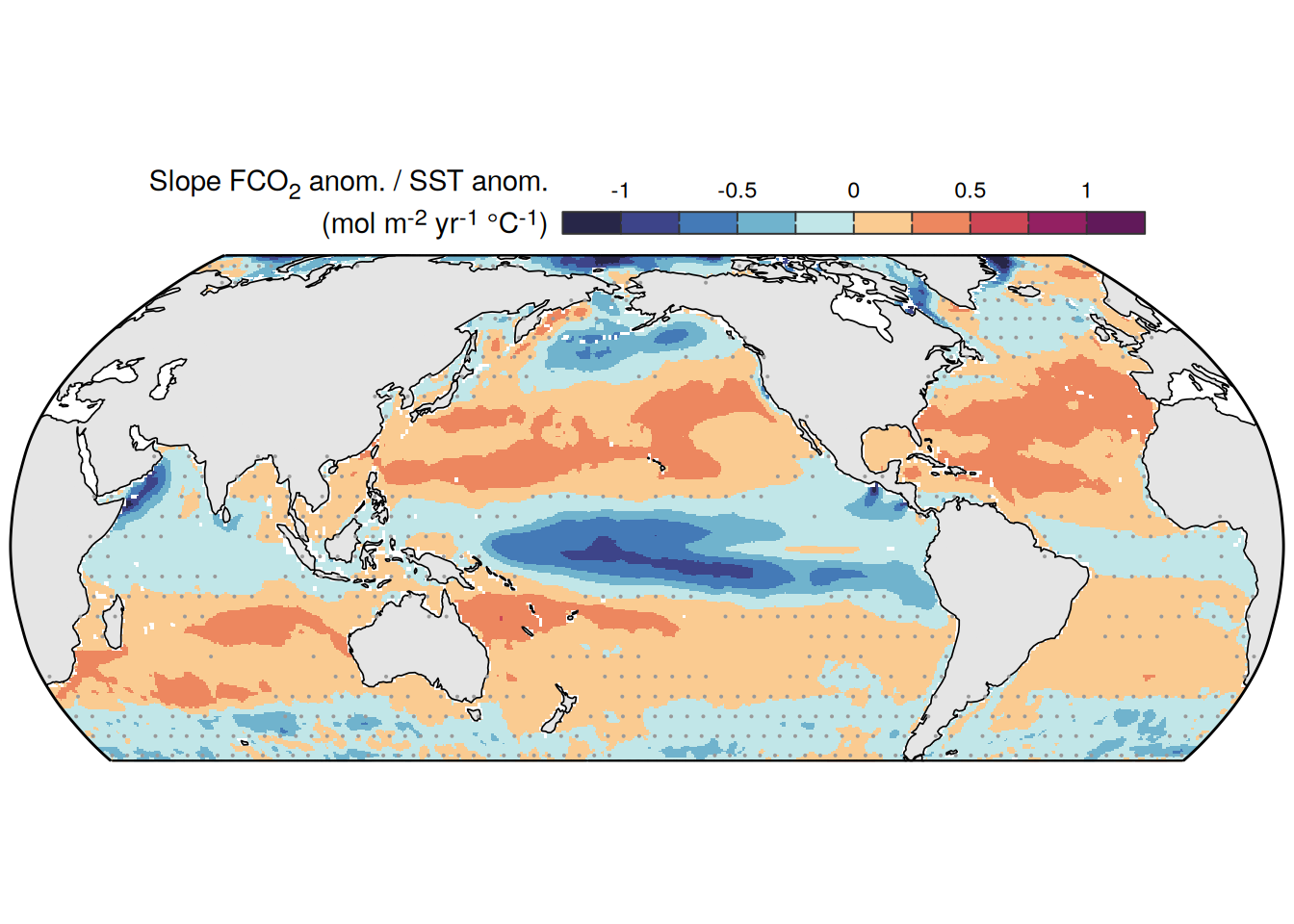
[[4]]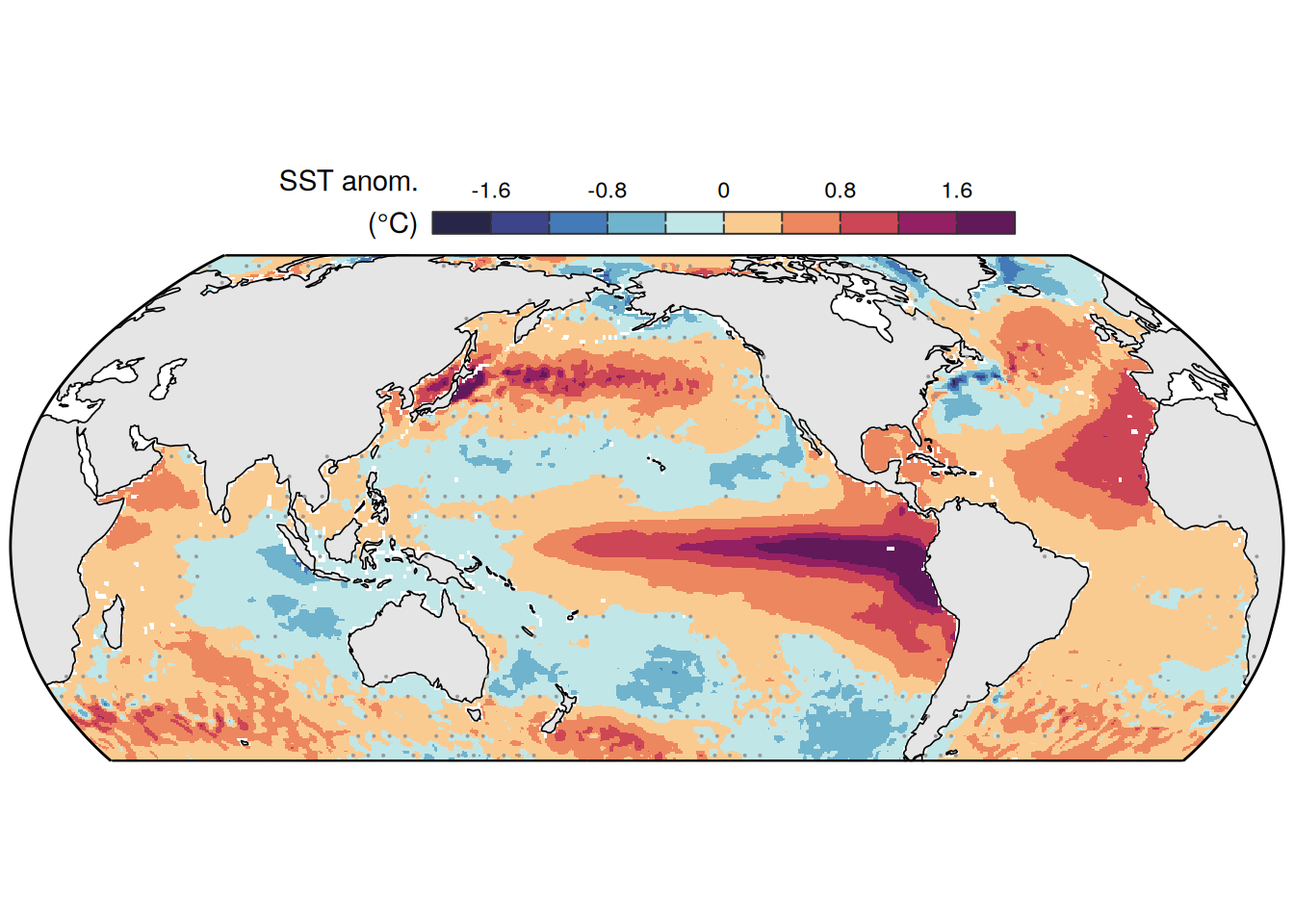
plot_list <- pco2_product_map_annual_anomaly_temperature_predict_ensemble %>%
  mutate(product = "Ensemble mean") %>%
  group_split(name) %>%
  map(
    ~ p_map_mdim_robinson(
      df = .x,
      df_uncertainty = pco2_product_map_annual_anomaly_temperature_predict_ensemble_uncertainty %>%
        filter(name == .x %>% distinct(name) %>% pull()),
      var = "resid_mean",
      legend_title = labels_breaks(.x %>% distinct(name))$i_legend_title,
      legend_position = "bottom",
      breaks = labels_breaks(.x %>% distinct(name))$i_breaks,
      n_labels = 2
    )
  )

ggsave(plot = wrap_plots(plot_list,
                         ncol = 2),
       width = 12,
       height = 6,
       filename = "../output/map_annual_anomaly_temperature_predict_ensemble.pdf")

rm(
  pco2_product_map_annual_anomaly_temperature_predict_ensemble,
  pco2_product_map_annual_anomaly_temperature_predict_ensemble_coarse,
  pco2_product_map_annual_anomaly_temperature_predict_ensemble_uncertainty
)

gc()
used (Mb) gc trigger (Mb) max used (Mb)
Ncells 3264434 174.4 7041390 376.1 7041390 376.1
Vcells 352827201 2691.9 600295772 4579.9 600295772 4579.9pco2_product_2024_map_annual_anomaly_temperature_predict_merge <-
bind_rows(
pco2_product_2024_map_annual_anomaly_temperature_predict %>%
pivot_longer(-c(product, year, lon, lat), values_to = "resid"),
pco2_product_map_annual_anomaly_temperature_predict %>%
filter(product %in% c("SOM-FFN", "CMEMS")) %>%
mutate(year = 2023)
)
pco2_product_2024_map_annual_anomaly_temperature_predict_merge %>%
filter(name == "slope") %>%
mutate(year = case_when(
year == "2023" ~ "1990-2022",
year == "2024" ~ "1990-2023",
TRUE ~ "none"
)) %>%
p_map_mdim_robinson(
var = "resid",
legend_title = "Slope FCO<sub>2</sub> anom. / SST anom.<br>(mol m<sup>-2</sup> yr<sup>-1</sup> °C<sup>-1</sup>)",
breaks = c(-Inf, seq(-1, 1, 0.25), Inf),
dim_row = "year",
dim_col = "product"
)
ggsave(width = 10,
height = 5,
dpi = 600,
filename = "../output/map_anomaly_correlation_2024.pdf")
pco2_product_2024_map_annual_anomaly_temperature_predict_merge %>%
filter(str_detect(name, "temperature")) %>%
p_map_mdim_robinson(
var = "resid",
legend_title = labels_breaks("temperature")$i_legend_title,
breaks = labels_breaks("temperature")$i_breaks,
dim_row = "year",
dim_col = "product"
)
ggsave(width = 10,
height = 5,
dpi = 600,
filename = "../output/map_anomaly_sst_2024.pdf")
pco2_product_2024_map_annual_anomaly_temperature_predict_merge %>%
filter(name == "fgco2") %>%
p_map_mdim_robinson(
var = "resid",
legend_title = labels_breaks("fgco2")$i_legend_title,
breaks = labels_breaks("fgco2")$i_breaks,
dim_row = "year",
dim_col = "product"
)
ggsave(width = 10,
height = 5,
dpi = 600,
filename = "../output/map_anomaly_flux_observed_2024.pdf")
pco2_product_2024_map_annual_anomaly_temperature_predict_merge %>%
filter(str_detect(name, "fgco2_predict")) %>%
p_map_mdim_robinson(
var = "resid",
legend_title = labels_breaks("fgco2_predict")$i_legend_title,
breaks = labels_breaks("fgco2_predict")$i_breaks,
dim_row = "year",
dim_col = "product"
)
ggsave(width = 10,
height = 5,
dpi = 600,
filename = "../output/map_anomaly_flux_predicted_2024.pdf")
plot_list <- pco2_product_2024_map_annual_anomaly_temperature_predict_merge %>%
filter(name %in% c("fgco2", "temperature"),
product == "SOM-FFN",
year == 2024) %>%
group_split(name) %>%
map(
~ p_map_mdim_robinson(
df = .x,
var = "resid",
legend_title = labels_breaks(.x %>% distinct(name))$i_legend_title,
legend_position = "top",
breaks = labels_breaks(.x %>% distinct(name))$i_breaks,
n_labels = 2
)
)
ggsave(plot = wrap_plots(plot_list,
ncol = 2,
byrow = FALSE),
width = 10,
height = 3,
dpi = 900,
filename = "../output/map_anomaly_SOM-FFN_2024.pdf")pco2_product_2024_map_annual_anomaly_temperature_predict_merge_ensemble <-
pco2_product_2024_map_annual_anomaly_temperature_predict_merge %>%
filter(year == "2024") %>%
fgroup_by(name, lon, lat) %>%
fsummarise(
resid_sd = fsd(resid),
resid_mean = fmean(resid),
n = fnobs(resid)
) %>%
filter(n == 2) %>%
select(-n)
pco2_product_2024_map_annual_anomaly_temperature_predict_merge_ensemble_coarse <-
m_grid_horizontal_coarse(pco2_product_2024_map_annual_anomaly_temperature_predict_merge_ensemble) %>%
fgroup_by(name, lon_grid, lat_grid) %>%
fsummarise(
resid_sd_coarse = fmean(resid_sd, na.rm = TRUE),
resid_mean_coarse = fmean(resid_mean, na.rm = TRUE)
) %>%
rename(lon = lon_grid, lat = lat_grid)
pco2_product_2024_map_annual_anomaly_temperature_predict_merge_ensemble_uncertainty <-
pco2_product_2024_map_annual_anomaly_temperature_predict_merge_ensemble_coarse %>%
mutate(signif_single = if_else(abs(resid_mean_coarse) < resid_sd_coarse, 0, 1)) %>%
select(lon, lat, name, signif_single) %>%
st_as_sf(coords = c("lon", "lat"), crs = "+proj=longlat")
pco2_product_2024_map_annual_anomaly_temperature_predict_merge_ensemble %>%
mutate(product = "Ensemble mean") %>%
group_split(name) %>%
# head(1) %>%
map(
~ p_map_mdim_robinson(
df = .x,
df_uncertainty = pco2_product_2024_map_annual_anomaly_temperature_predict_merge_ensemble_uncertainty %>%
filter(name == .x %>% distinct(name) %>% pull()),
var = "resid_mean",
legend_title = labels_breaks(.x %>% distinct(name))$i_legend_title,
breaks = labels_breaks(.x %>% distinct(name))$i_breaks,
n_labels = 2
)
)
plot_list <- pco2_product_2024_map_annual_anomaly_temperature_predict_merge_ensemble %>%
mutate(product = "Ensemble mean") %>%
group_split(name) %>%
map(
~ p_map_mdim_robinson(
df = .x,
df_uncertainty = pco2_product_2024_map_annual_anomaly_temperature_predict_merge_ensemble_uncertainty %>%
filter(name == .x %>% distinct(name) %>% pull()),
var = "resid_mean",
legend_title = labels_breaks(.x %>% distinct(name))$i_legend_title,
legend_position = "top",
breaks = labels_breaks(.x %>% distinct(name))$i_breaks,
n_labels = 2
)
)
ggsave(plot = wrap_plots(plot_list,
ncol = 2),
width = 20,
height = 10,
dpi = 900,
filename = "../output/map_annual_anomaly_temperature_predict_ensemble_2024.pdf")
rm(
pco2_product_2024_map_annual_anomaly_temperature_predict_merge_ensemble,
pco2_product_2024_map_annual_anomaly_temperature_predict_merge_ensemble_coarse,
pco2_product_2024_map_annual_anomaly_temperature_predict_merge_ensemble_uncertainty
)
gc()Monthly means
2023 anomaly
pco2_product_map_monthly_anomaly <-
  inner_join(
    biome_mask_print,
    pco2_product_map_monthly_anomaly
  )
pco2_product_map_monthly_anomaly %>%
filter(name %in% name_core,
year == 2023) %>%
group_split(name) %>%
head(1) %>%
map(
~ map +
geom_tile(data = .x,
aes(lon, lat, fill = resid)) +
scale_fill_gradientn(
colours = warm_cool_gradient,
rescaler = ~ scales::rescale_mid(.x, mid = 0),
name = labels_breaks(.x %>% distinct(name))$i_legend_title,
limits = c(quantile(.x$resid, .01), quantile(.x$resid, .99)),
oob = squish
) +
theme(legend.title = element_markdown()) +
facet_grid(month ~ product) +
guides(
fill = guide_colorbar(
barheight = unit(0.3, "cm"),
barwidth = unit(6, "cm"),
ticks = TRUE,
ticks.colour = "grey20",
frame.colour = "grey20",
label.position = "top",
direction = "horizontal"
)
) +
theme(legend.title = element_markdown(),
legend.position = "top")
)pco2_product_map_monthly_anomaly_ensemble <-
pco2_product_map_monthly_anomaly %>%
filter(year == 2023,
product %in% pco2_product_list) %>%
fgroup_by(name, lon, lat, month) %>%
fsummarise(
resid_sd = fsd(resid),
resid_mean = fmean(resid),
n = fnobs(resid)
) %>%
filter(n == length(pco2_product_list)) %>%
select(-n)
pco2_product_map_monthly_anomaly_ensemble_coarse <-
m_grid_horizontal_coarse(pco2_product_map_monthly_anomaly_ensemble) %>%
fgroup_by(name, month, lon_grid, lat_grid) %>%
fsummarise(resid_sd_coarse = fmean(resid_sd, na.rm = TRUE),
resid_mean_coarse = fmean(resid_mean, na.rm = TRUE)) %>%
rename(lon = lon_grid, lat = lat_grid)
pco2_product_map_monthly_anomaly_ensemble <-
left_join(
pco2_product_map_monthly_anomaly_ensemble,
pco2_product_map_monthly_anomaly_ensemble_coarse
)
pco2_product_map_monthly_anomaly_ensemble %>%
filter(name %in% name_core) %>%
mutate(month = as.character(month),
month = fct_inorder(month)) %>%
group_split(name) %>%
head(1) %>%
map(
~ p_map_mdim_robinson(
df = .x,
var = "resid_mean",
dim_wrap = "month",
legend_title = labels_breaks(.x %>% distinct(name))$i_legend_title,
breaks = labels_breaks(.x %>% distinct(name))$i_breaks
)
)[[1]]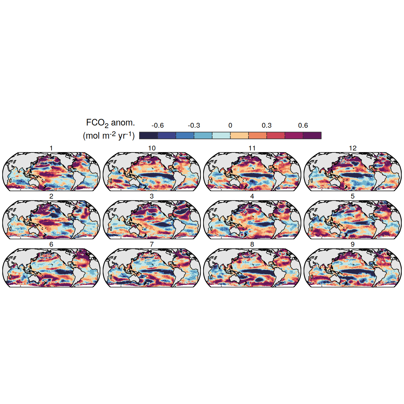
| Version | Author | Date |
|---|---|---|
| 42ecae0 | jens-daniel-mueller | 2025-03-13 |
| 17f843d | jens-daniel-mueller | 2025-03-10 |
| fb85a52 | jens-daniel-mueller | 2025-03-10 |
| ae5b6a4 | jens-daniel-mueller | 2025-03-10 |
| b9e8f8c | jens-daniel-mueller | 2025-03-10 |
| 9fe7d3d | jens-daniel-mueller | 2025-03-02 |
| 417f35d | jens-daniel-mueller | 2025-02-28 |
| d532d40 | jens-daniel-mueller | 2025-02-28 |
| 518e3d0 | jens-daniel-mueller | 2025-02-27 |
rm(
  pco2_product_map_monthly_anomaly_ensemble,
  pco2_product_map_monthly_anomaly_ensemble_coarse
)

gc()
used (Mb) gc trigger (Mb) max used (Mb)
Ncells 3215984 171.8 7041390 376.1 7041390 376.1
Vcells 308449420 2353.3 600295772 4579.9 600295772 4579.9fCO2 decomposition
pco2_product_map_monthly_fCO2_decomposition <-
  inner_join(pco2_product_map_monthly_fCO2_decomposition,
             biome_mask_print)
pco2_product_map_monthly_fCO2_decomposition %>%
filter(year == 2023) %>%
group_split(product) %>%
# head(1) %>%
map(
~ map +
geom_tile(data = .x,
aes(lon, lat, fill = resid)) +
labs(title = .x$product) +
scale_fill_gradientn(
colours = warm_cool_gradient,
rescaler = ~ scales::rescale_mid(.x, mid = 0),
name = labels_breaks("sfco2"),
limits = c(quantile(.x$resid, .01), quantile(.x$resid, .99)),
oob = squish
) +
facet_grid(month ~ name,
labeller = labeller(name = x_axis_labels)) +
guides(
fill = guide_colorbar(
barheight = unit(0.3, "cm"),
barwidth = unit(6, "cm"),
ticks = TRUE,
ticks.colour = "grey20",
frame.colour = "grey20",
label.position = "top",
direction = "horizontal"
)
) +
theme(legend.title = element_markdown(),
legend.position = "top")
)
pco2_product_map_monthly_fCO2_decomposition %>%
filter(year == 2023,
product %in% pco2_product_list) %>%
group_by(name, lon, lat, month) %>%
summarize(
resid_sd = sd(resid),
resid_mean = mean(resid),
n = n()
) %>%
ungroup() %>%
filter(n == length(pco2_product_list)) %>%
select(-n) %>%
mutate(product = "Ensemble mean") %>%
group_split(product) %>%
# head(1) %>%
map(
~ map +
geom_tile(data = .x,
aes(lon, lat, fill = resid_mean)) +
# geom_point(
# data = .x %>% filter(abs(resid_mean) < resid_sd),
# aes(lon, lat, shape = "Ensemble mean\n< StDev"),
# col = "grey"
# ) +
scale_fill_gradientn(
colours = warm_cool_gradient,
rescaler = ~ scales::rescale_mid(.x, mid = 0),
name = labels_breaks("sfco2"),,
limits = c(quantile(.x$resid_mean, .01), quantile(.x$resid_mean, .99)),
oob = squish
) +
scale_shape_manual(values = 46, name = "") +
facet_grid(month ~ name,
labeller = labeller(name = x_axis_labels)) +
guides(
fill = guide_colorbar(
barheight = unit(0.3, "cm"),
barwidth = unit(6, "cm"),
ticks = TRUE,
ticks.colour = "grey20",
frame.colour = "grey20",
label.position = "top",
direction = "horizontal"
)
) +
theme(legend.title = element_markdown(),
legend.position = "top")
)pco2_product_map_annual_fCO2_decomposition <-
pco2_product_map_monthly_fCO2_decomposition %>%
select(product, year, lat, lon, name, resid) %>%
fgroup_by(product, year, lat, lon, name) %>%
fmean()
gc() used (Mb) gc trigger (Mb) max used (Mb)
Ncells 3185489 170.2 7041390 376.1 7041390 376.1
Vcells 282217790 2153.2 600295772 4579.9 600295772 4579.9pco2_product_map_annual_fCO2_decomposition %>%
filter(year == 2023) %>%
select(-year) %>%
relocate(lon, lat) %>%
# mutate(name = str_remove(name, "sfco2_")) %>%
p_map_mdim_robinson(
var = "resid",
dim_col = "name",
dim_row = "product",
legend_title = labels_breaks("sfco2")$i_legend_title,
breaks = 2 * (labels_breaks("sfco2")$i_breaks),
n_labels = 2
)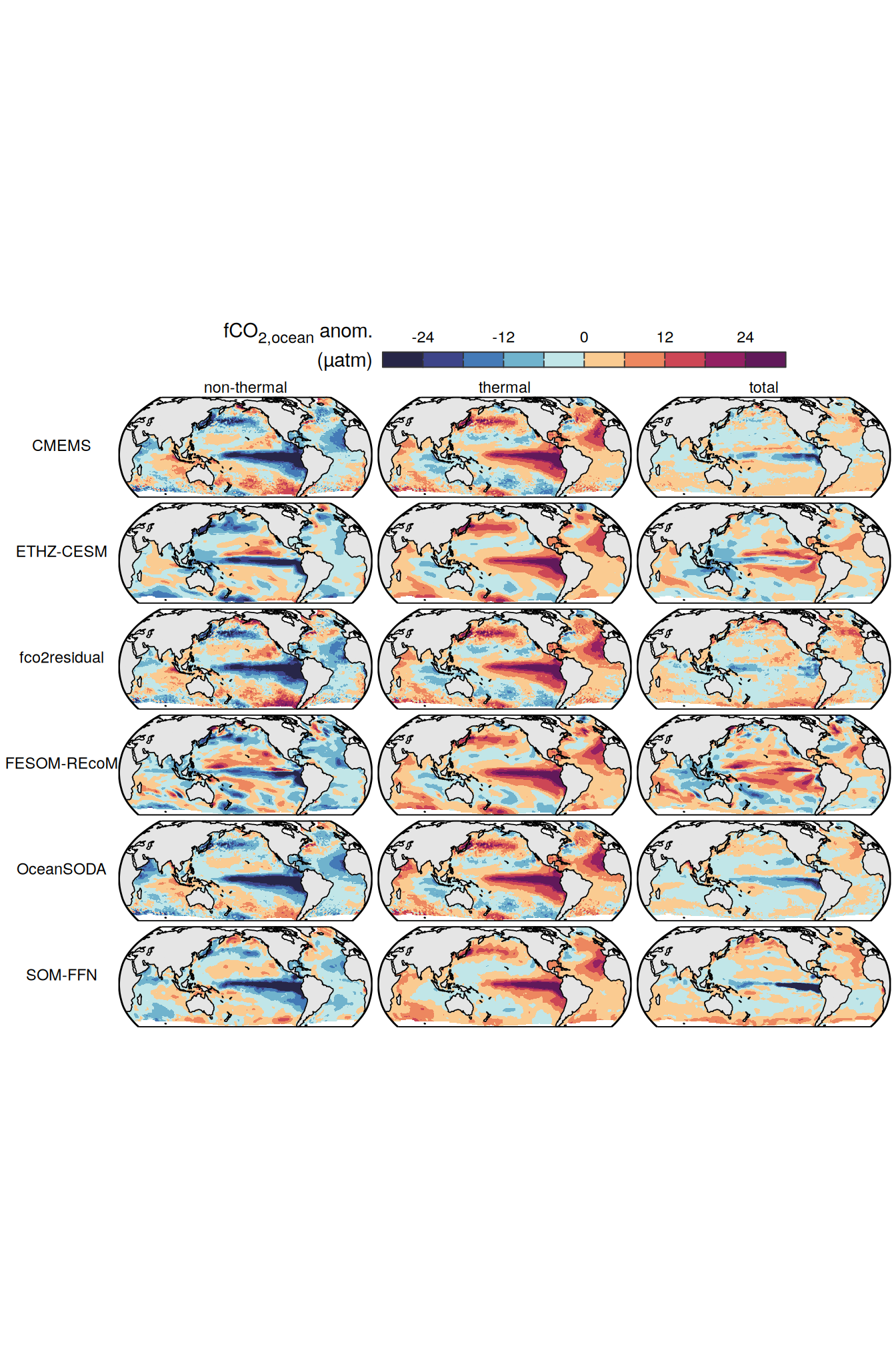
| Version | Author | Date |
|---|---|---|
| 17f843d | jens-daniel-mueller | 2025-03-10 |
| fb85a52 | jens-daniel-mueller | 2025-03-10 |
| ae5b6a4 | jens-daniel-mueller | 2025-03-10 |
| b9e8f8c | jens-daniel-mueller | 2025-03-10 |
| 9fe7d3d | jens-daniel-mueller | 2025-03-02 |
| 9276be7 | jens-daniel-mueller | 2025-03-02 |
| 417f35d | jens-daniel-mueller | 2025-02-28 |
| d532d40 | jens-daniel-mueller | 2025-02-28 |
| 518e3d0 | jens-daniel-mueller | 2025-02-27 |
pco2_product_map_annual_fCO2_decomposition_ensemble <-
  pco2_product_map_annual_fCO2_decomposition %>%
  filter(product %in% pco2_product_list, year == 2023) %>%
  group_by(name, lon, lat) %>%
  summarize(resid_sd = sd(resid),
            resid_mean = mean(resid),
            n = n()) %>%
  ungroup() %>%
  filter(n == length(pco2_product_list)) %>%
  select(-n)


pco2_product_map_annual_fCO2_decomposition_ensemble_coarse <-
  m_grid_horizontal_coarse(pco2_product_map_annual_fCO2_decomposition_ensemble) %>%
  fgroup_by(name, lon_grid, lat_grid) %>%
  fsummarise(resid_sd_coarse = fmean(resid_sd, na.rm = TRUE),
             resid_mean_coarse = fmean(resid_mean, na.rm = TRUE)) %>%
  rename(lon = lon_grid, lat = lat_grid)


pco2_product_map_annual_fCO2_decomposition_ensemble_uncertainty <-
  pco2_product_map_annual_fCO2_decomposition_ensemble_coarse %>%
  mutate(signif_single = if_else(abs(resid_mean_coarse) < resid_sd_coarse, 0, 1)) %>%
  select(lon, lat, name, signif_single) %>%
  st_as_sf(coords = c("lon", "lat"), crs = "+proj=longlat")


pco2_product_map_annual_fCO2_decomposition_ensemble %>%
  select(lon, lat, name, resid_mean) %>%
  mutate(name = fct_relevel(name,
                            c("sfco2_therm", "sfco2_nontherm"))) %>%
  p_map_mdim_robinson(
    df_uncertainty = pco2_product_map_annual_fCO2_decomposition_ensemble_uncertainty,
    var = "resid_mean",
    legend_title = labels_breaks("sfco2")$i_legend_title,
    breaks = 2*(labels_breaks("sfco2")$i_breaks),
    dim_wrap = "name",
    n_col = 1,
    n_labels = 2
  )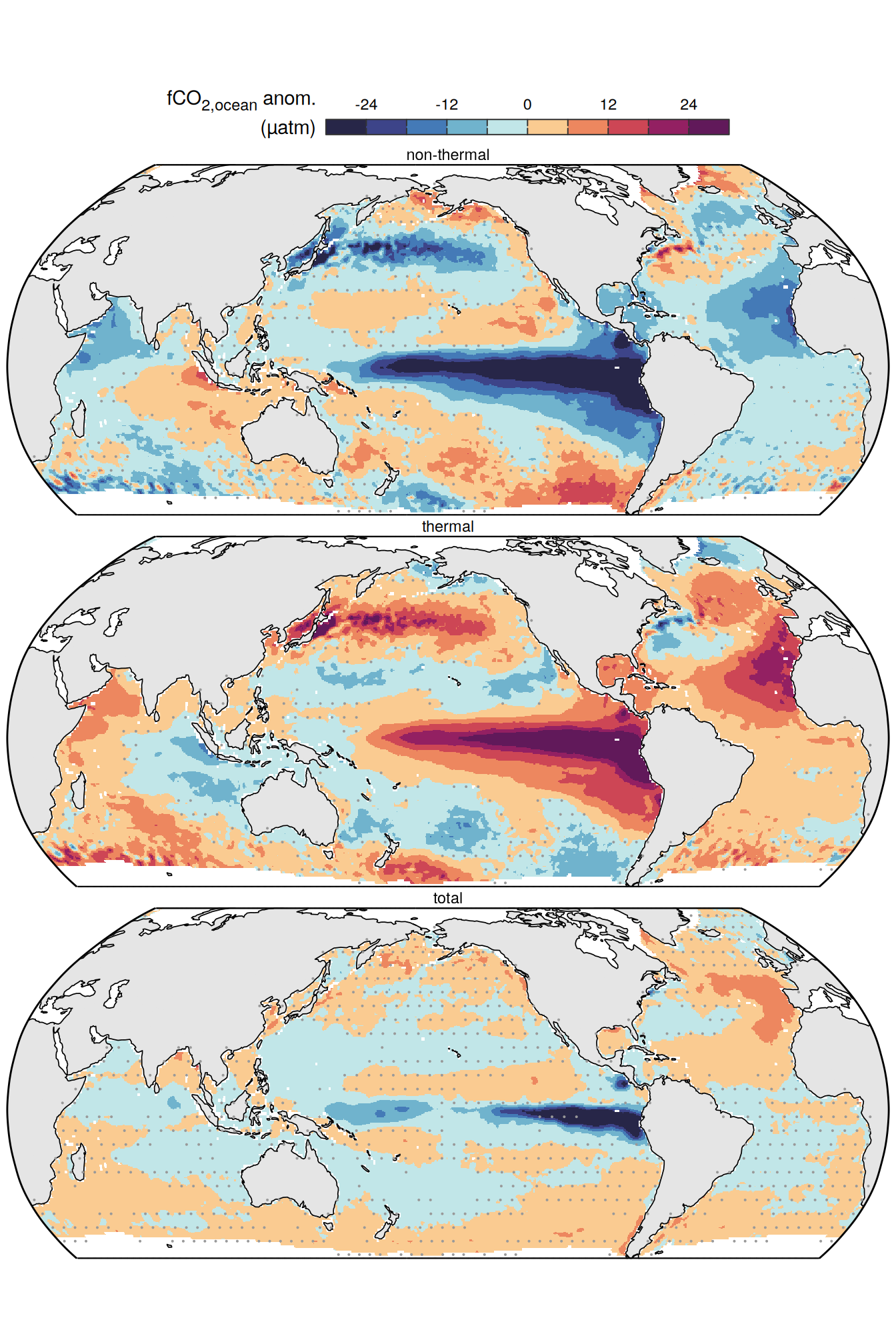
| Version | Author | Date |
|---|---|---|
| 17f843d | jens-daniel-mueller | 2025-03-10 |
| fb85a52 | jens-daniel-mueller | 2025-03-10 |
| ae5b6a4 | jens-daniel-mueller | 2025-03-10 |
| b9e8f8c | jens-daniel-mueller | 2025-03-10 |
| 9fe7d3d | jens-daniel-mueller | 2025-03-02 |
| 417f35d | jens-daniel-mueller | 2025-02-28 |
| d532d40 | jens-daniel-mueller | 2025-02-28 |
| 518e3d0 | jens-daniel-mueller | 2025-02-27 |
ggsave(width = 5,
       height = 7,
       dpi = 1200,
       filename = "../output/map_anomaly_fco2_decomposition_ensemble_mean_pco2_products.pdf")

grDevices::cairo_pdf(
  "../output/Fig3_edf.pdf",
  width = 5.5,
  height = 7.5,
  onefile = TRUE
)


pco2_product_map_annual_fCO2_decomposition_ensemble %>%
  select(lon, lat, name, resid_mean) %>%
  mutate(name = fct_relevel(name,
                            c("sfco2_therm", "sfco2_nontherm"))) %>%
  p_map_mdim_robinson(
    df_uncertainty = pco2_product_map_annual_fCO2_decomposition_ensemble_uncertainty,
    var = "resid_mean",
    legend_title = labels_breaks("sfco2")$i_legend_title,
    breaks = 2*(labels_breaks("sfco2")$i_breaks),
    dim_wrap = "name",
    n_col = 1,
    n_labels = 2
  )

dev.off()
png
2 pco2_product_map_annual_fCO2_decomposition_ensemble %>%
select(lon, lat, name, resid_mean) %>%
mutate(name = fct_relevel(name,
c("sfco2_therm", "sfco2_nontherm"))) %>%
p_map_mdim_robinson(
df_uncertainty = pco2_product_map_annual_fCO2_decomposition_ensemble_uncertainty,
var = "resid_mean",
legend_title = labels_breaks("sfco2")$i_legend_title,
breaks = labels_breaks("sfco2")$i_breaks,
dim_wrap = "name",
n_col = 1,
n_labels = 2
)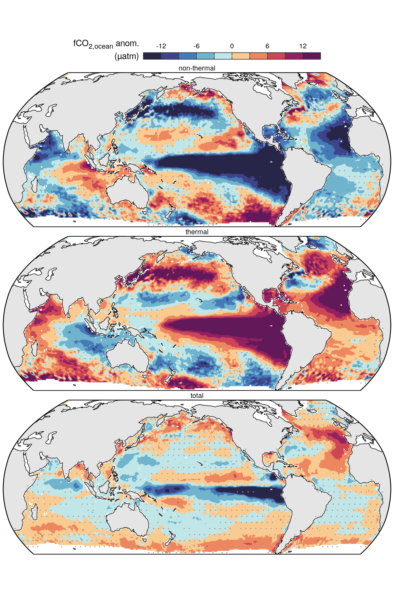
| Version | Author | Date |
|---|---|---|
| 265b0a8 | jens-daniel-mueller | 2025-06-06 |
ggsave(width = 5,
       height = 7,
       dpi = 1200,
       filename = "../output/map_anomaly_fco2_decomposition_ensemble_mean_pco2_products_breaks.pdf")
Flux attribution
pco2_product_map_monthly_flux_attribution <-
  inner_join(pco2_product_map_monthly_flux_attribution, biome_mask_print)
# pco2_product_map_monthly_flux_attribution <-
# flux_attribution(pco2_product_map_monthly_anomaly,
# year, month, lon, lat)
pco2_product_map_monthly_flux_attribution %>%
filter(year == 2023) %>%
drop_na() %>%
group_split(product) %>%
# head(1) %>%
map(
~ map +
geom_tile(data = .x,
aes(lon, lat, fill = resid)) +
labs(subtitle = .x$product) +
scale_fill_gradientn(
colours = warm_cool_gradient,
rescaler = ~ scales::rescale_mid(.x, mid = 0),
name = labels_breaks("fgco2"),
limits = c(quantile(.x$resid, .01), quantile(.x$resid, .99)),
oob = squish
) +
theme(legend.title = element_markdown(),
legend.position = "bottom") +
facet_grid(month ~ name,
labeller = labeller(name = x_axis_labels)) +
guides(
fill = guide_colorbar(
barheight = unit(0.3, "cm"),
barwidth = unit(6, "cm"),
ticks = TRUE,
ticks.colour = "grey20",
frame.colour = "grey20",
label.position = "top",
direction = "horizontal"
)
) +
theme(legend.title = element_markdown(),
legend.position = "top",
strip.text.x.top = element_markdown())
)
pco2_product_map_monthly_flux_attribution %>%
filter(year == 2023) %>%
drop_na() %>%
filter(product %in% pco2_product_list) %>%
group_by(name, lon, lat, month) %>%
summarize(
resid_sd = sd(resid),
resid_mean = mean(resid),
n = n()
) %>%
ungroup() %>%
filter(n == length(pco2_product_list)) %>%
select(-n) %>%
mutate(product = "Ensemble mean") %>%
drop_na() %>%
group_split(product) %>%
# head(1) %>%
map(
~ map +
geom_tile(data = .x,
aes(lon, lat, fill = resid_mean)) +
# geom_point(data = .x %>% filter(abs(resid_mean) < resid_sd),
# aes(lon, lat, shape = "Ensemble mean\n< StDev"))+
scale_fill_gradientn(
colours = warm_cool_gradient,
rescaler = ~ scales::rescale_mid(.x, mid = 0),
name = labels_breaks("fgco2"),
limits = c(quantile(.x$resid_mean, .01), quantile(.x$resid_mean, .99)),
oob = squish
)+
scale_shape_manual(values = 46, name = "") +
theme(legend.title = element_markdown(),
legend.position = "bottom") +
facet_grid(month ~ name,
labeller = labeller(name = x_axis_labels)) +
guides(
fill = guide_colorbar(
barheight = unit(0.3, "cm"),
barwidth = unit(6, "cm"),
ticks = TRUE,
ticks.colour = "grey20",
frame.colour = "grey20",
label.position = "top",
direction = "horizontal"
)
) +
theme(
legend.title = element_markdown(),
legend.position = "top",
strip.text.x.top = element_markdown()
)
)pco2_product_map_annual_flux_attribution <-
pco2_product_map_monthly_flux_attribution %>%
group_by(product, year, lat, lon, name) %>%
summarise(resid = mean(resid, na.rm = TRUE)) %>%
ungroup()
pco2_product_map_annual_flux_attribution %>%
filter(year == 2023) %>%
select(-year) %>%
relocate(lon, lat) %>%
# mutate(name = str_remove_all(name, "_")) %>%
p_map_mdim_robinson(
var = "resid",
dim_row = "product",
dim_col = "name",
legend_title = labels_breaks("fgco2")$i_legend_title,
breaks = labels_breaks("fgco2")$i_breaks,
n_labels = 2
)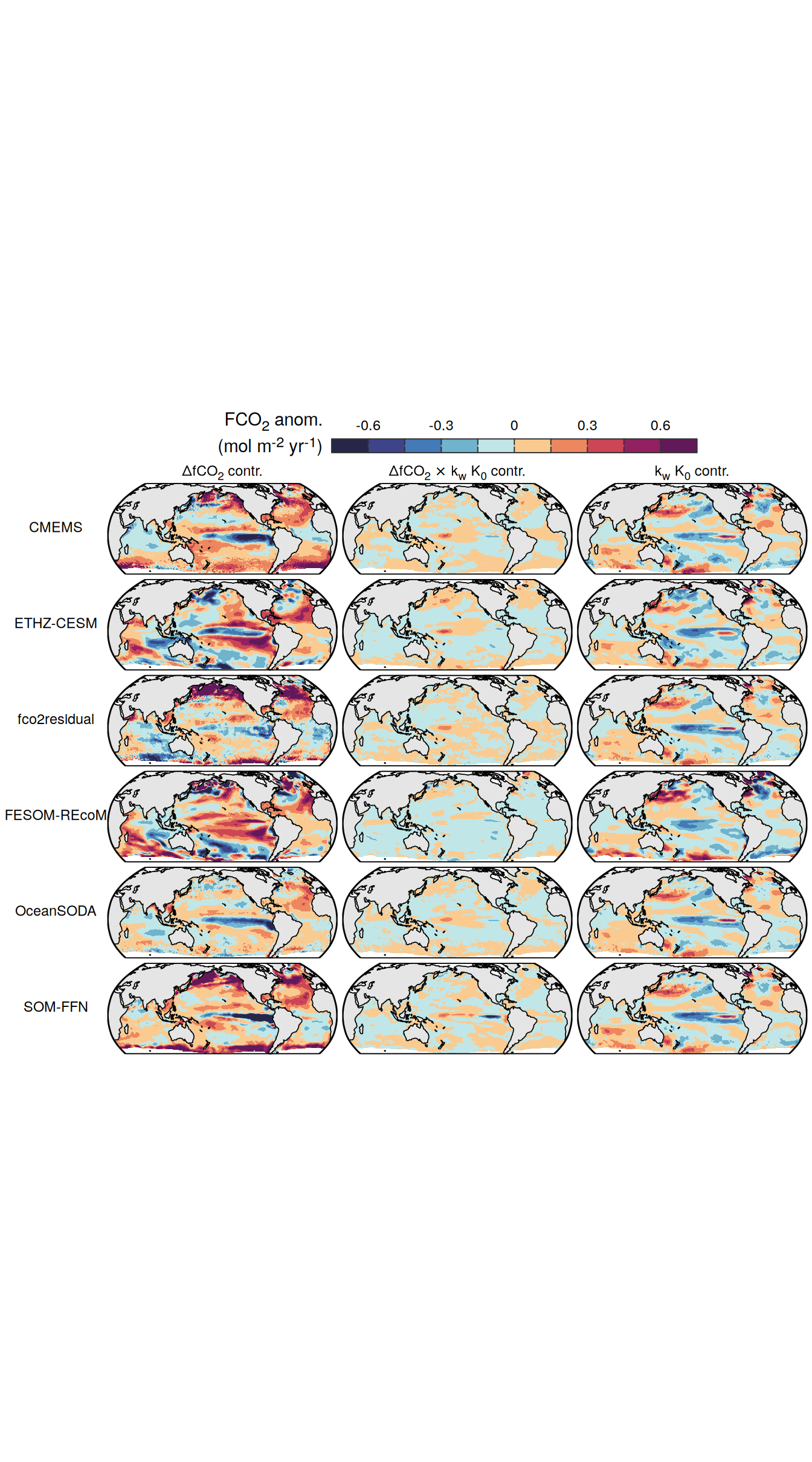
| Version | Author | Date |
|---|---|---|
| 42ecae0 | jens-daniel-mueller | 2025-03-13 |
| 17f843d | jens-daniel-mueller | 2025-03-10 |
| fb85a52 | jens-daniel-mueller | 2025-03-10 |
| ae5b6a4 | jens-daniel-mueller | 2025-03-10 |
| b9e8f8c | jens-daniel-mueller | 2025-03-10 |
| 9fe7d3d | jens-daniel-mueller | 2025-03-02 |
| 9276be7 | jens-daniel-mueller | 2025-03-02 |
| 417f35d | jens-daniel-mueller | 2025-02-28 |
| d532d40 | jens-daniel-mueller | 2025-02-28 |
| 518e3d0 | jens-daniel-mueller | 2025-02-27 |
pco2_product_map_annual_flux_attribution_ensemble <-
pco2_product_map_annual_flux_attribution %>%
  filter(year == 2023,
         product %in% pco2_product_list) %>%
  group_by(name, lon, lat) %>%
  summarize(
    resid_sd = sd(resid),
    resid_mean = mean(resid),
    n = n()
  ) %>%
  ungroup() %>%
  filter(n == length(pco2_product_list)) %>%
  select(-n) %>%
  drop_na()

pco2_product_map_annual_flux_attribution_ensemble_coarse <-
  m_grid_horizontal_coarse(pco2_product_map_annual_flux_attribution_ensemble) %>%
  fgroup_by(name, lon_grid, lat_grid) %>%
  fsummarise(resid_sd_coarse = fmean(resid_sd, na.rm = TRUE),
             resid_mean_coarse = fmean(resid_mean, na.rm = TRUE)) %>%
  rename(lon = lon_grid, lat = lat_grid)


pco2_product_map_annual_flux_attribution_ensemble_uncertainty <-
  pco2_product_map_annual_flux_attribution_ensemble_coarse %>%
  mutate(signif_single = if_else(abs(resid_mean_coarse) < resid_sd_coarse, 0, 1)) %>%
  select(lon, lat, name, signif_single) %>%
  st_as_sf(coords = c("lon", "lat"), crs = "+proj=longlat")


pco2_product_map_annual_flux_attribution_ensemble %>%
  select(lon, lat, name, resid_mean) %>%
  p_map_mdim_robinson(
    df_uncertainty = pco2_product_map_annual_flux_attribution_ensemble_uncertainty,
    var = "resid_mean",
    legend_title = labels_breaks("fgco2")$i_legend_title,
    breaks = labels_breaks("fgco2")$i_breaks,
    dim_wrap = "name",
    n_col = 1,
    n_labels = 2
  )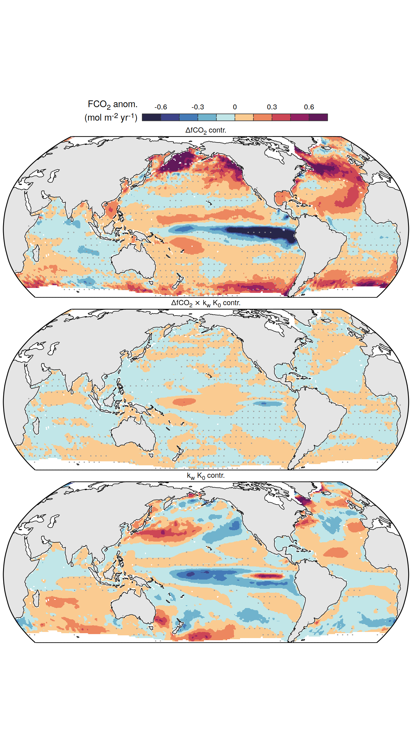
| Version | Author | Date |
|---|---|---|
| 42ecae0 | jens-daniel-mueller | 2025-03-13 |
| 17f843d | jens-daniel-mueller | 2025-03-10 |
| fb85a52 | jens-daniel-mueller | 2025-03-10 |
| ae5b6a4 | jens-daniel-mueller | 2025-03-10 |
| b9e8f8c | jens-daniel-mueller | 2025-03-10 |
| 9fe7d3d | jens-daniel-mueller | 2025-03-02 |
| 417f35d | jens-daniel-mueller | 2025-02-28 |
| d532d40 | jens-daniel-mueller | 2025-02-28 |
| 518e3d0 | jens-daniel-mueller | 2025-02-27 |
ggsave(width = 5,
       height = 7,
       dpi = 1200,
       filename = "../output/map_anomaly_flux_attribution_ensemble_mean_pco2_products.pdf")

grDevices::cairo_pdf(
  "../output/Fig3_acb.pdf",
  width = 5.5,
  height = 7.5,
  onefile = TRUE
)


pco2_product_map_annual_flux_attribution_ensemble %>%
  select(lon, lat, name, resid_mean) %>%
  p_map_mdim_robinson(
    df_uncertainty = pco2_product_map_annual_flux_attribution_ensemble_uncertainty,
    var = "resid_mean",
    legend_title = labels_breaks("fgco2")$i_legend_title,
    breaks = labels_breaks("fgco2")$i_breaks,
    dim_wrap = "name",
    n_col = 1,
    n_labels = 2
  )

dev.off()
png
2 Hovmoeller plots
The following Hovmoeller plots show the anomalies from the prediction of a linear/quadratic fit to the data from 1990 to 2022.
Hovmoeller plots are presented as monthly means. Note that the predictions for the monthly Hovmoeller plots are done individually for each month, such the mean seasonal anomaly from the annual mean is removed.
Monthly means
Anomalies
pco2_product_hovmoeller_monthly_anomaly <-
pco2_product_hovmoeller_monthly_anomaly %>%
  filter(name %in% c("fgco2_hov", "temperature"))

pco2_product_hovmoeller_monthly_anomaly %>%
  group_split(name) %>%
  # head(2) %>%
  map(
    ~ ggplot(data = .x,
             aes(decimal, lat, fill = resid)) +
      geom_raster() +
      scale_fill_gradientn(
        colours = warm_cool_gradient,
        rescaler = ~ scales::rescale_mid(.x, mid = 0),
        name = labels_breaks(.x %>% distinct(name))$i_legend_title,
        limits = c(quantile(.x$resid,.01),quantile(.x$resid,.99)),
        oob = squish
      ) +
      theme(legend.title = element_markdown()) +
      coord_cartesian(expand = 0) +
      labs(title = "Monthly mean anomalies",
           y = "Latitude") +
      theme(axis.title.x = element_blank()) +
      facet_wrap(~ product, ncol = 1)
  )
[[1]]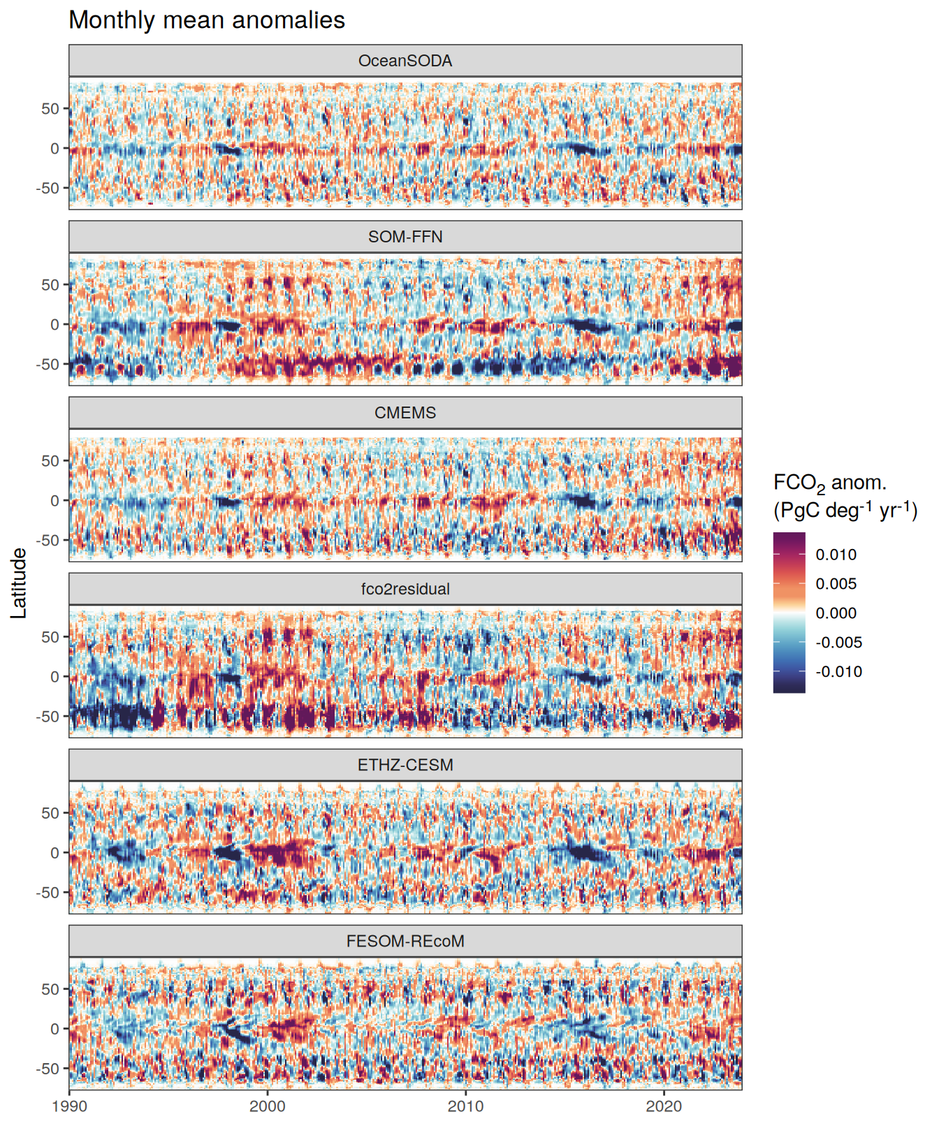
| Version | Author | Date |
|---|---|---|
| 265b0a8 | jens-daniel-mueller | 2025-06-06 |
[[2]]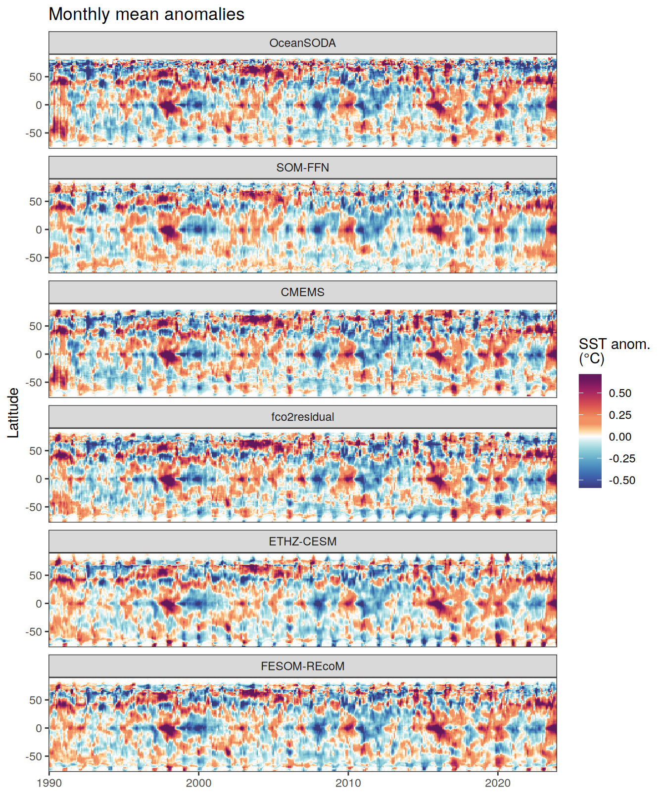
| Version | Author | Date |
|---|---|---|
| 265b0a8 | jens-daniel-mueller | 2025-06-06 |
pco2_product_hovmoeller_monthly_anomaly_ensemble <-
  pco2_product_hovmoeller_monthly_anomaly %>%
  filter(product %in% pco2_product_list) %>%
  group_by(name, decimal, lat) %>%
  summarize(
    resid_range = max(resid) - min(resid),
    resid_sd = sd(resid),
    resid_mean = mean(resid),
    n = n()
  ) %>%
  ungroup() %>%
  filter(n == 4)


pco2_product_hovmoeller_monthly_anomaly_ensemble %>%
  mutate(product = "Ensemble mean") %>%
  group_split(name) %>%
  # head(1) %>%
  map(
    ~ ggplot(data = .x,
             aes(decimal, lat, fill = resid_mean)) +
      geom_raster() +
      scale_fill_gradientn(
        colours = warm_cool_gradient,
        rescaler = ~ scales::rescale_mid(.x, mid = 0),
        name = labels_breaks(.x %>% distinct(name))$i_legend_title,
        limits = c(quantile(.x$resid_mean, .01), quantile(.x$resid_mean, .99)),
        oob = squish
      ) +
      theme(legend.title = element_markdown()) +
      coord_cartesian(expand = 0) +
      labs(title = "Monthly mean anomalies",
           y = "Latitude") +
      theme(axis.title.x = element_blank()) +
      facet_wrap( ~ product, ncol = 1)
  )
[[1]]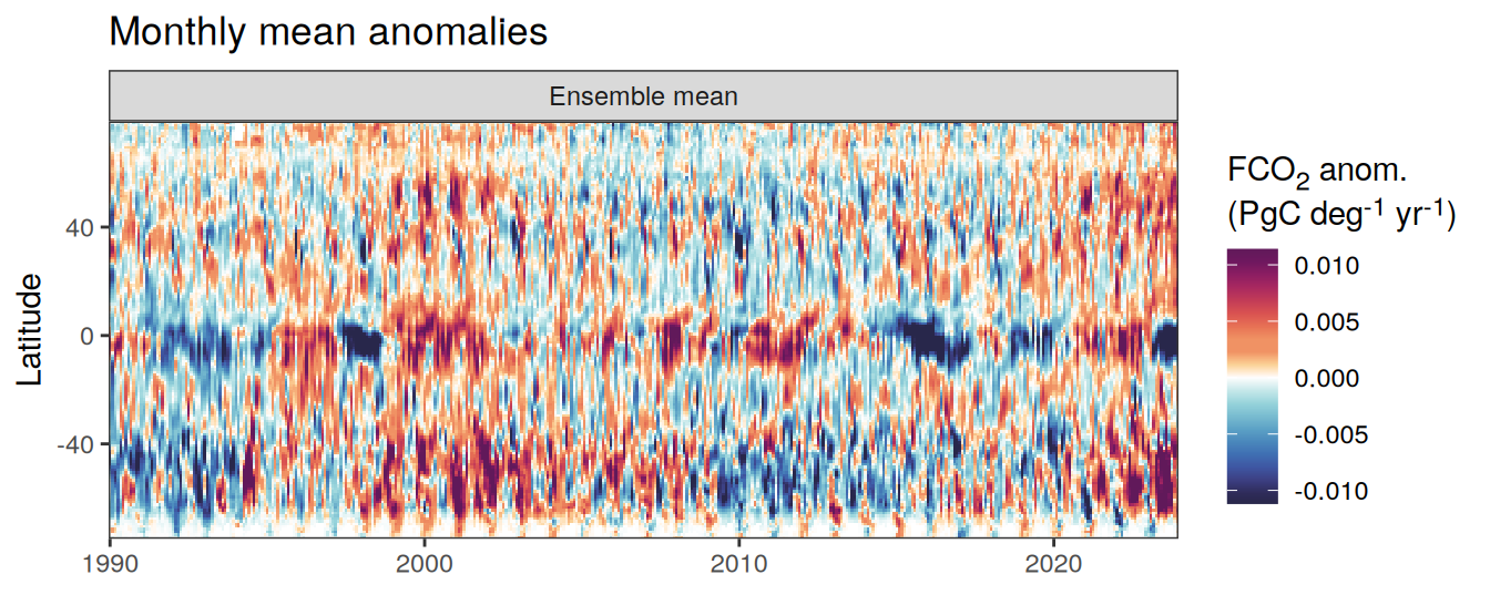
| Version | Author | Date |
|---|---|---|
| 265b0a8 | jens-daniel-mueller | 2025-06-06 |
[[2]]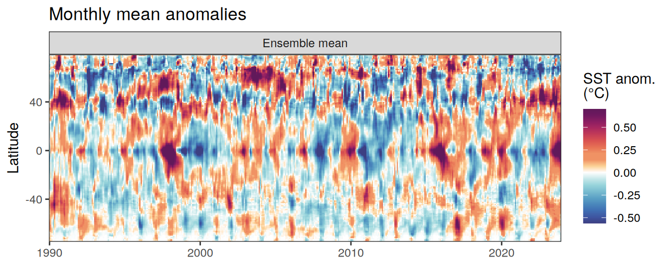
| Version | Author | Date |
|---|---|---|
| 265b0a8 | jens-daniel-mueller | 2025-06-06 |
pco2_product_hovmoeller_annual_anomaly_ensemble <-
pco2_product_hovmoeller_monthly_anomaly_ensemble %>%
  mutate(year = floor(decimal)) %>%
  group_by(year, lat, name) %>%
  summarise(resid_mean = mean(resid_mean),
            resid_sd = mean(resid_sd)) %>%
  ungroup()


p_hov_sst <- pco2_product_hovmoeller_annual_anomaly_ensemble %>%
  filter(name == "temperature") %>%
  ggplot(aes(resid_mean, lat, group = year)) +
  geom_vline(xintercept = 0) +
  geom_path(data = . %>% filter(!year %in% c(2023, 1997, 2015)),
            aes(col = "Other years\n1990-2022"),
            alpha = 0.5) +
  scale_color_manual(values = "grey60", name = "X") +
  scale_fill_manual(values = "grey60", name = "X") +
  new_scale_fill() +
  new_scale_color() +
  # geom_path(data = . %>% filter(year %in% 2002:2007),
  #           aes(col = "2002-2007"),
  #           alpha = 0.5) +
  # scale_color_manual(values = cold_color, name = "X") +
  # scale_fill_manual(values = cold_color, name = "X") +
  # new_scale_fill() +
  # new_scale_color() +
  geom_path(data = . %>% filter(year %in% c(2023, 1997, 2015)),
            aes(col = as.factor(year)),
            linewidth = 1) +
  scale_fill_manual(values = rev(warm_cool_gradient[c(17, 13, 20)]),
                    guide = guide_legend(reverse = TRUE, order = 2)) +
  scale_color_manual(values = rev(warm_cool_gradient[c(17, 13, 20)]),
                     guide = guide_legend(reverse = TRUE, order = 2)) +
  labs(x = labels_breaks("temperature")$i_legend_title,
       y = "Latitude (°N)") +
  scale_y_continuous(breaks = seq(-60, 60, 30), expand = c(0,0)) +
  theme_bw() +
  theme(axis.title = element_markdown(),
        legend.title = element_blank(),
        panel.grid.minor = element_blank())

p_hov_fgco2 <- pco2_product_hovmoeller_annual_anomaly_ensemble %>%
  filter(name == "fgco2_hov") %>%
  ggplot(aes(resid_mean, lat, group = year)) +
  geom_vline(xintercept = 0) +
  geom_path(data = . %>% filter(!year %in% c(2023, 1997, 2015)),
            aes(col = "Other years\n1990-2022"),
            alpha = 0.5) +
  scale_color_manual(values = "grey60", name = "X") +
  scale_fill_manual(values = "grey60", name = "X") +
  new_scale_fill() +
  new_scale_color() +
  # geom_path(data = . %>% filter(year %in% 2002:2007),
  #           aes(col = "2002-2007"),
  #           alpha = 0.5) +
  # scale_color_manual(values = cold_color, name = "X") +
  # scale_fill_manual(values = cold_color, name = "X") +
  # new_scale_fill() +
  # new_scale_color() +
  geom_path(data = . %>% filter(year %in% c(2023, 1997, 2015)),
            aes(col = as.factor(year)),
            linewidth = 1) +
  scale_fill_manual(values = rev(warm_cool_gradient[c(17, 13, 20)]),
                    guide = guide_legend(reverse = TRUE, order = 2)) +
  scale_color_manual(values = rev(warm_cool_gradient[c(17, 13, 20)]),
                     guide = guide_legend(reverse = TRUE, order = 2)) +
  labs(x = labels_breaks("fgco2_hov")$i_legend_title,
       y = "Latitude (°N)") +
  scale_y_continuous(breaks = seq(-60, 60, 30), expand = c(0,0)) +
  theme_bw() +
  theme(axis.title = element_markdown(),
        legend.title = element_blank(),
        axis.title.y = element_blank(),
        axis.text.y = element_blank(),
        panel.grid.minor = element_blank())


p_hov_sst + p_hov_fgco2  +
   plot_layout(guides = 'collect')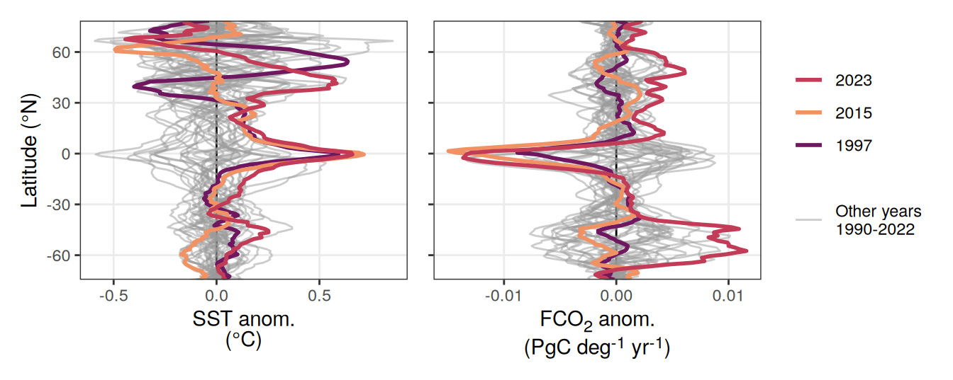
| Version | Author | Date |
|---|---|---|
| 265b0a8 | jens-daniel-mueller | 2025-06-06 |
ggsave(width = 7,
       height = 7,
       dpi = 600,
       filename = "../output/zonal_mean_anomaly_sst_co2flux_ensemble_mean_pco2_products.pdf")
pco2_product_2024_hovmoeller_annual_anomaly <-
pco2_product_2024_hovmoeller_monthly_anomaly %>%
filter(name %in% c("temperature", "fgco2_hov")) %>%
group_by(product, year, lat, name) %>%
summarise(resid = mean(resid)) %>%
ungroup()
pco2_product_2024_hovmoeller_annual_anomaly %>%
ggplot(aes(resid, lat, group = year)) +
geom_vline(xintercept = 0) +
geom_path(data = . %>% filter(!year %in% 2023:2024),
aes(col = "1990-2022"),
alpha = 0.5) +
scale_color_manual(values = "grey60", name = "X") +
scale_fill_manual(values = "grey60", name = "X") +
new_scale_fill() +
new_scale_color() +
geom_path(data = . %>% filter(year %in% 2023:2024),
aes(col = as.factor(year)),
linewidth = 1) +
scale_fill_manual(values = warm_cool_gradient[c(17, 20)],
guide = guide_legend(reverse = TRUE, order = 2)) +
scale_color_manual(values = warm_cool_gradient[c(17, 20)],
guide = guide_legend(reverse = TRUE, order = 2)) +
# labs(x = labels_breaks("temperature")$i_legend_title,
# y = "Latitude (°N)") +
scale_y_continuous(breaks = seq(-60, 60, 30), expand = c(0,0)) +
theme_bw() +
facet_grid(product ~ name, scales = "free_x") +
theme(axis.title = element_markdown(),
legend.title = element_blank(),
panel.grid.minor = element_blank())
p_hov_sst <- pco2_product_2024_hovmoeller_annual_anomaly %>%
filter(name == "temperature",
product == "SOM-FFN") %>%
ggplot(aes(resid, lat, group = year)) +
geom_vline(xintercept = 0) +
geom_ribbon(data = . %>% filter(year %in% 2023),
aes(xmin = 0, xmax = pmax(0, resid)),
alpha = 0.9,
fill = "grey70") +
geom_ribbon(data = . %>% filter(year %in% 2023),
aes(xmax = 0, xmin = pmin(0, resid)),
alpha = 0.9,
fill = "grey70") +
geom_path(data = . %>% filter(year %in% 2023:2024),
aes(col = as.factor(year)),
linewidth = 1) +
scale_fill_manual(values = warm_cool_gradient[c(17, 20)],
guide = guide_legend(reverse = TRUE, order = 2)) +
scale_color_manual(values = warm_cool_gradient[c(17, 20)],
guide = guide_legend(reverse = TRUE, order = 2)) +
scale_y_continuous(breaks = seq(-60,60,30),
name = "Lat (°N)",
limits = c(-54,76),
expand = c(0,0)) +
scale_x_continuous(breaks = seq(-0.5,0.5,0.5),
name = labels_breaks("temperature")$i_legend_title,
position = "top") +
theme_classic() +
theme(
legend.position = "none",
axis.title.x = element_markdown(),
axis.text.y = element_blank(),
axis.ticks.y = element_blank(),
axis.title.y = element_blank(),
axis.line.y = element_blank()
)
p_hov_fgco2 <- pco2_product_2024_hovmoeller_annual_anomaly %>%
filter(name == "fgco2_hov",
product == "SOM-FFN") %>%
ggplot(aes(resid*1000, lat, group = year)) +
geom_vline(xintercept = 0) +
geom_ribbon(data = . %>% filter(year %in% 2023),
aes(xmin = 0, xmax = pmax(0, resid*1000)),
alpha = 0.9,
fill = "grey70") +
geom_ribbon(data = . %>% filter(year %in% 2023),
aes(xmax = 0, xmin = pmin(0, resid*1000)),
alpha = 0.9,
fill = "grey70") +
geom_path(data = . %>% filter(year %in% 2023:2024),
aes(col = as.factor(year)),
linewidth = 1) +
scale_fill_manual(values = warm_cool_gradient[c(17, 20)],
guide = guide_legend(reverse = TRUE, order = 2)) +
scale_color_manual(values = warm_cool_gradient[c(17, 20)],
guide = guide_legend(reverse = TRUE, order = 2)) +
scale_y_continuous(breaks = seq(-60,60,30),
name = "Lat (°N)",
limits = c(-54,76),
expand = c(0,0)) +
scale_x_continuous(breaks = seq(-20,20,20),
name = str_replace(
labels_breaks("fgco2_hov")$i_legend_title,
"PgC", "TgC"
),
position = "top") +
theme_classic() +
theme(
legend.position = "none",
axis.title.x = element_markdown(),
axis.text.y = element_blank(),
axis.ticks.y = element_blank(),
axis.title.y = element_blank(),
axis.line.y = element_blank()
)
p_hov_sst + p_hov_fgco2 +
plot_layout(guides = 'collect')
ggsave(width = 2.2,
height = 3.5,
dpi = 900,
filename = "../output/zonal_mean_anomaly_sst_co2flux_ensemble_mean_pco2_products_2024.pdf")left_join(
pco2_product_hovmoeller_monthly_anomaly_ensemble,
pco2_product_hovmoeller_monthly_anomaly
) %>%
mutate(resid_offset = resid - resid_mean) %>%
group_split(name) %>%
# head(1) %>%
map(
~ ggplot(data = .x,
aes(decimal, lat, fill = resid_offset)) +
geom_raster() +
scale_fill_gradientn(
colours = warm_cool_gradient,
rescaler = ~ scales::rescale_mid(.x, mid = 0),
name = labels_breaks(.x %>% distinct(name))$i_legend_title,
limits = c(quantile(.x$resid_mean, .01), quantile(.x$resid_mean, .99)),
oob = squish
) +
theme(legend.title = element_markdown()) +
coord_cartesian(expand = 0)+
labs(title = "Monthly offset from ensemble mean anomalies",
y = "Latitude") +
theme(axis.title.x = element_blank()) +
facet_wrap( ~ product, ncol = 1)
)Regional means and integrals
The following plots show biome-, super biome- or global- averaged/integrated values of each variable as provided through the fCO2 product, represented here as the anomalies from the prediction of a linear/quadratic fit to the data from 1990 to 2022.
Anomalies are presented relative to the predicted annual mean of each year, hence preserving the seasonality.
Annual anomalies
pco2_product_biome_annual_anomaly_ensemble <-
  pco2_product_biome_annual_anomaly %>%
  filter(product %in% pco2_product_list) %>%
  group_by(year, name, biome) %>%
  summarise(resid_sd = sd(resid),
            resid = mean(resid),
            value = mean(value),
            fit = mean(fit)) %>%
  ungroup()

# fit lin. reg. model fgco2 anomaly vs SST anomaly per biome
# excluding anomaly year from fit

pco2_product_biome_annual_anomaly %>%
  filter(
    name %in% c("fgco2_int", "temperature"),
    biome == "Global non-polar",
    product %in% pco2_product_list
  ) %>%
  select(year, product, name, resid) %>%
  ggplot(aes(year, resid, col = product)) +
  geom_hline(yintercept = 0) +
  geom_path() +
  facet_wrap(~name, scales = "free_y")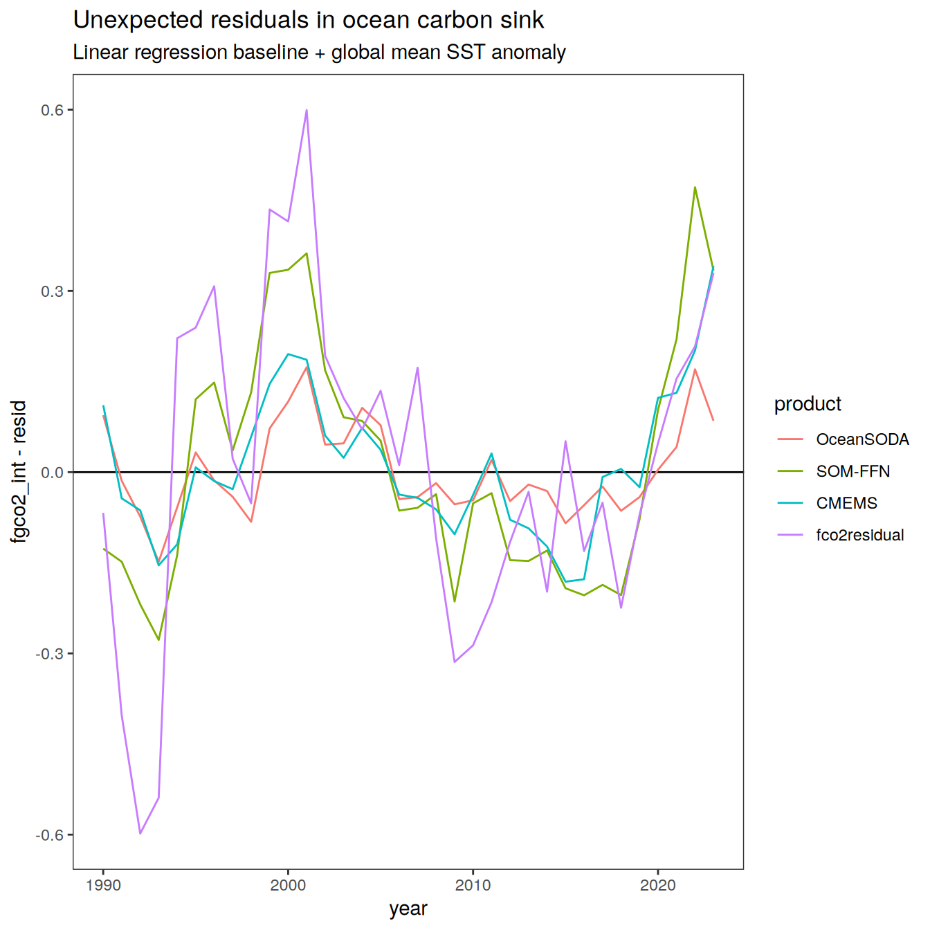
lm_fgco2_sst <- pco2_product_biome_annual_anomaly %>%
  filter(
    name %in% c("fgco2_int", "temperature"),
    biome == "Global non-polar",
    product %in% pco2_product_list
  ) %>%
  select(year, product, name, resid) %>%
  pivot_wider(values_from = resid) %>%
  nest(data = -product) %>%
  mutate(fit = map(data, ~ lm(
    formula = fgco2_int ~ temperature,
    data = .x %>% filter(year != 2023)
  )))

# predict fgco2 anomaly from SST anomaly per biome
# include anomaly year for prediction

lm_fgco2_sst <- lm_fgco2_sst %>%
  mutate(resid = map2(fit, data, predict)) %>%
  unnest(c(data, resid))

# extract regression coefficients

lm_fgco2_sst <- lm_fgco2_sst %>%
  mutate(coeff = map(fit, coefficients)) %>%
  select(-fit) %>%
  rename(temperature_obs = temperature) %>%
  unnest_wider(coeff) %>%
  rename(intercept = `(Intercept)`,
         slope = temperature,
         temperature = temperature_obs)


lm_fgco2_sst %>%
  filter(year == 2023) %>%
  select(-fgco2_int) %>%
  mutate(across(c(slope, temperature, resid), ~ round(.x, 2)),
         across(c(intercept), ~ signif(.x, 2))) %>%
  write_csv("../output/lm_fgco2_sst.csv")


# compute unexpected (predicted vs observed) flux anomalies

lm_fgco2_sst %>%
  select(product, year, fgco2_int, resid) %>%
  pivot_longer(c(fgco2_int, resid)) %>%
  ggplot(aes(year, value, col = product)) +
  geom_hline(yintercept = 0) +
  geom_path() +
  facet_wrap(~name) +
  labs(title = "Unexpected residuals in ocean carbon sink",
       subtitle = "Linear regression baseline + global mean SST anomaly")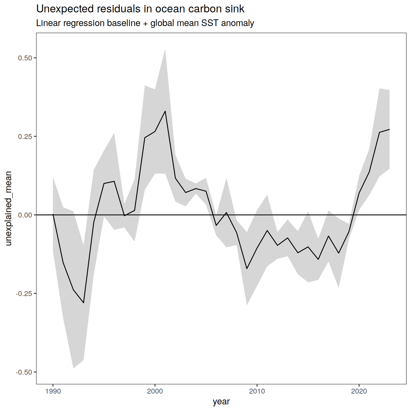
lm_fgco2_sst %>%
  ggplot(aes(year, fgco2_int-resid, col = product)) +
  geom_hline(yintercept = 0) +
  geom_path() +
  labs(title = "Unexpected residuals in ocean carbon sink",
       subtitle = "Linear regression baseline + global mean SST anomaly")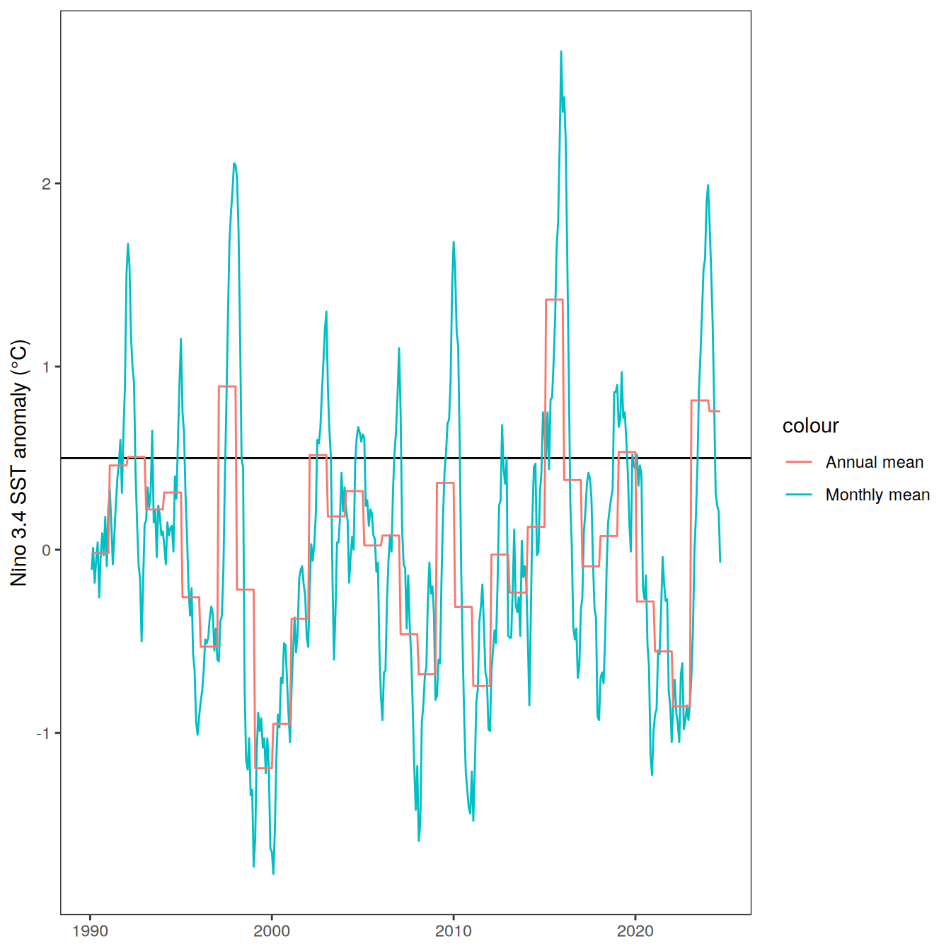
pco2_product_biome_annual_anomaly_lm_fgco2_sst <-
  inner_join(
    pco2_product_biome_annual_anomaly %>%
      filter(
        name %in% c("fgco2_int"),
        biome == "Global non-polar",
        product %in% pco2_product_list
      ) %>%
      select(year, product, baseline = fit),
    lm_fgco2_sst %>%
      select(year, product, resid)
  )


lm_fgco2_sst <-
  lm_fgco2_sst %>%
  group_by(year) %>%
  summarise(
    resid_sd = sd(resid),
    resid_mean = mean(resid),
    unexplained_sd = sd(fgco2_int - resid),
    unexplained_mean = mean(fgco2_int - resid),
    temperature_sd = sd(temperature),
    temperature_mean = mean(temperature)
  ) %>%
  ungroup()


lm_fgco2_sst %>%
  ggplot(aes(year, unexplained_mean,
             ymin = unexplained_mean - unexplained_sd,
             ymax = unexplained_mean + unexplained_sd)) +
  geom_hline(yintercept = 0) +
  geom_ribbon(alpha = 0.2) +
  geom_path() +
  labs(title = "Unexpected residuals in ocean carbon sink",
       subtitle = "Linear regression baseline + global mean SST anomaly")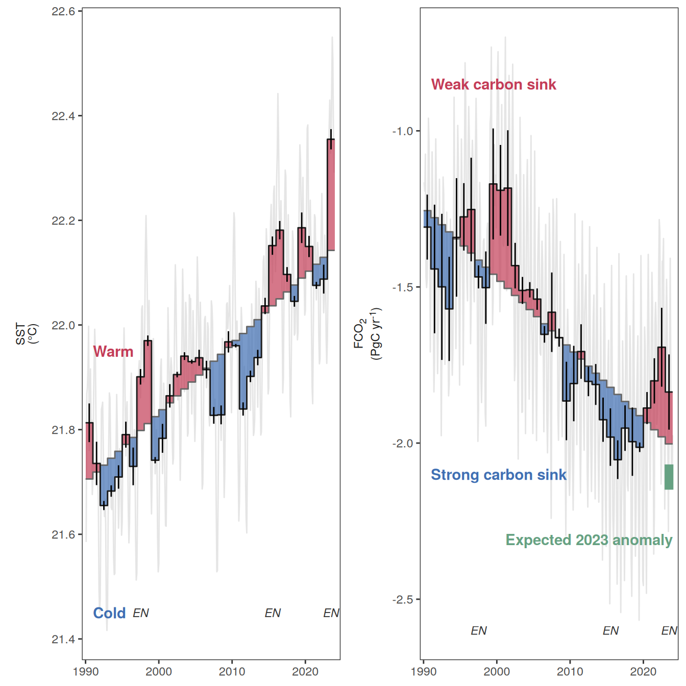
pco2_product_biome_annual_anomaly_ensemble_lm_fgco2_sst <-
  inner_join(
    lm_fgco2_sst %>%
      select(-starts_with("unex")),
    pco2_product_biome_annual_anomaly_ensemble %>%
      filter(name %in% c("fgco2_int"), biome == "Global non-polar") %>%
      select(year, name, fit)
  ) %>%
  mutate(fgco2_predict = resid_mean + fit) %>%
  select(-fit)

nino_sst %>%
  filter(year >= 1990) %>%
  ggplot(aes(year + month/12, resid)) +
  geom_hline(yintercept = 0.5) +
  geom_path(aes(col = "Monthly mean")) +
  geom_path(data = . %>%
              group_by(year) %>%
              mutate(resid = mean(resid)) %>%
              ungroup(),
            aes(col = "Annual mean")) +
  labs(y = "Nino 3.4 SST anomaly (°C)") +
  theme(axis.title.x = element_blank())
bind_rows(
  pco2_product_biome_annual_anomaly_ensemble,
  pco2_product_biome_annual_anomaly_ensemble %>%
    filter(year == max(year)) %>%
    mutate(year = year + 1) %>%
    select(-c(resid, resid_sd))
) %>%
  filter(name %in% c("fgco2_int", "temperature"), biome == "Global non-polar") %>%
  mutate(name = fct_rev(as.factor(name))) %>%
  ggplot() +
  geom_path(
    data = pco2_product_biome_monthly_anomaly %>%
      filter(
        product %in% pco2_product_list,
        name %in% c("fgco2_int", "temperature"),
        biome == "Global non-polar"
      ) %>%
      group_by(year, month, name, biome) %>%
      summarise(value = mean(value)) %>%
      ungroup(),
    aes(year + month / 12, value),
    col = "grey90"
  ) +
  geom_rect(
    data = pco2_product_biome_annual_anomaly_ensemble_lm_fgco2_sst %>%
      filter(year %in% 2023),
    aes(xmin = year, xmax = year + 1, ymin = fgco2_predict - resid_sd,
        ymax = fgco2_predict + resid_sd),
    fill = trend_color, col = trend_color
  ) +
  geom_text(
    data = pco2_product_biome_annual_anomaly_ensemble_lm_fgco2_sst %>%
      filter(year %in% c(2023)),
    aes(x = year + 1, y = fgco2_predict - 0.2, label = "Expected 2023 anomaly"),
    hjust = 1,
    fontface = "bold",
    col = trend_color
  ) +
  geom_text(
    data = . %>%
      filter(year == 1991, name == "temperature"),
    aes(x = year, y = 21.95, label = "Warm"),
    hjust = 0,
    fontface = "bold",
    col = warm_color
  ) +
  geom_text(
    data = . %>%
      filter(year == 1991, name == "temperature"),
    aes(x = year, y = 21.45, label = "Cold"),
    hjust = 0,
    fontface = "bold",
    col = cold_color
  ) +
  geom_text(
    data = . %>%
      filter(year == 1991, name == "fgco2_int"),
    aes(x = year, y = -0.85, label = "Weak carbon sink"),
    hjust = 0,
    fontface = "bold",
    col = warm_color
  ) +
  geom_text(
    data = . %>%
      filter(year == 1991, name == "fgco2_int"),
    aes(x = year, y = -2.1, label = "Strong carbon sink"),
    hjust = 0,
    fontface = "bold",
    col = cold_color
  ) +
  geom_text(
    data = . %>%
      filter(year %in% c(1997, 2015, 2023), name == "fgco2_int"),
    aes(
      x = year + 0.5,
      y = -2.6,
      label = "EN"
    ), size = 3, fontface = "italic", col = "grey20") +
  geom_text(
    data = . %>%
      filter(year %in% c(1997, 2015, 2023), name == "temperature"),
    aes(
      x = year + 0.5,
      y = 21.45,
      label = "EN"
    ), size = 3, fontface = "italic", col = "grey20") +
  geom_rect(
    data = . %>% filter(year != max(year)),
    aes(
      xmin = year,
      xmax = year + 1,
      ymin = fit,
      ymax = value,
      fill = as.factor(sign(-resid))
    ),
    alpha = 0.7
  ) +
  geom_step(aes(year, fit, col = "Baseline")) +
  geom_step(aes(year, value, col = "Observed")) +
  geom_linerange(aes(
    x = year + 0.5,
    ymin = value - resid_sd,
    ymax = value + resid_sd,
    linetype = "Product SD"
  )) +
  scale_color_manual(values = c("grey40", "grey10"), name = "Annual means") +
  scale_fill_manual(
    values = c(warm_color, cold_color),
    labels = c("positive", "negative"),
    name = "Anomalies"
  ) +
  scale_linetype(name = "Anomaly uncertainty") +
  guides(
    color = guide_legend(order = 1),
    fill = guide_legend(order = 2),
    linetype = guide_legend(order = 3)
  ) +
  scale_x_continuous(limits = c(1989.5, 2024.8), expand = c(0, 0)) +
  facet_wrap(
    . ~ name,
    scales = "free_y",
    strip.position = "left",
    labeller = labeller(name = x_axis_labels_abs)
    # switch = "y"
  )+
  labs(x = "Year") +
  theme(
    axis.title.y = element_blank(),
    axis.title.x = element_blank(),
    strip.text.y.left = element_markdown(),
    strip.placement = "outside",
    strip.background.y = element_blank(),
    legend.position = "none",
    legend.direction = "vertical"
  )
ggsave(width = 10,
       height = 2,
       dpi = 600,
       filename = "../output/Fig1_ab.pdf")

pco2_product_biome_annual_anomaly_ensemble_presentation <-
  bind_rows(
    pco2_product_biome_annual_anomaly_ensemble,
    pco2_product_biome_annual_anomaly_ensemble %>%
      filter(year == max(year)) %>%
      mutate(year = year + 1) %>%
      select(-c(resid, resid_sd))
  ) %>%
  filter(name %in% c("fgco2_int", "temperature"),
         biome == "Global non-polar")


pco2_product_biome_annual_anomaly_ensemble_presentation <-
  pco2_product_biome_annual_anomaly_ensemble_presentation %>%
  mutate(fit = case_when(
    name == "fgco2_int" & year == max(year) ~ fit - 0.022639,
    name == "temperature" & year == max(year) ~ fit + 0.01324,
    TRUE ~ fit
  ))

pco2_product_biome_annual_anomaly_ensemble_presentation <-
  bind_rows(
    pco2_product_biome_annual_anomaly_ensemble_presentation,
    pco2_product_biome_annual_anomaly_ensemble_presentation %>%
      filter(year == max(year)) %>%
      mutate(year = year + 1) %>%
      select(-c(resid, resid_sd, value))
  )

pco2_product_biome_annual_anomaly_ensemble_presentation %>%
  mutate(name = fct_rev(as.factor(name))) %>%
  ggplot() +
  geom_path(
    data = pco2_product_biome_monthly_anomaly %>%
      filter(
        product %in% pco2_product_list,
        name %in% c("fgco2_int", "temperature"),
        biome == "Global non-polar"
      ) %>%
      group_by(year, month, name, biome) %>%
      summarise(value = mean(value)) %>%
      ungroup(),
    aes(year + month / 12, value),
    col = "grey90"
  ) +
  # geom_rect(
  #   data = pco2_product_biome_annual_anomaly_ensemble_lm_fgco2_sst %>%
  #     filter(year %in% 2023),
  #   aes(xmin = year, xmax = year + 1, ymin = fgco2_predict - resid_sd,
  #       ymax = fgco2_predict + resid_sd),
  #   fill = trend_color, col = trend_color
  # ) +
  # geom_text(
  #   data = pco2_product_biome_annual_anomaly_ensemble_lm_fgco2_sst %>%
  #     filter(year %in% c(2023)),
  #   aes(x = year + 1, y = fgco2_predict - 0.2, label = "Expected 2023 anomaly"),
  #   hjust = 1,
  #   fontface = "bold",
  #   col = trend_color
  # ) +
  geom_rect(
    data = . %>% filter(year != max(year)),
    aes(
      xmin = year,
      xmax = year + 1,
      ymin = fit,
      ymax = value,
      fill = as.factor(sign(-resid))
    ),
    alpha = 0.7
  ) +
  geom_step(aes(year, fit, col = "Baseline")) +
  geom_point(data = . %>% filter(year == max(year), name == "fgco2_int"),
             aes(year-0.5, fit+0.65,fill = as.factor(sign(-1))),
             shape = 21, size = 2) +
  geom_step(aes(year, value, col = "Observed")) +
  geom_linerange(aes(
    x = year + 0.5,
    ymin = value - resid_sd,
    ymax = value + resid_sd,
    linetype = "Product SD"
  )) +
  scale_color_manual(values = c("grey40", "grey10"), name = "Annual means") +
  scale_fill_manual(
    values = c(warm_color, cold_color),
    labels = c("positive", "negative"),
    name = "Anomalies",
    na.value = "transparent"
  ) +
  scale_linetype(name = "Anomaly uncertainty") +
  guides(
    color = guide_legend(order = 1),
    fill = guide_legend(order = 2),
    linetype = guide_legend(order = 3)
  ) +
  scale_x_continuous(limits = c(1989.5, 2025.8), expand = c(0, 0)) +
  facet_wrap(
    . ~ name,
    scales = "free_y",
    strip.position = "left",
    labeller = labeller(name = x_axis_labels_abs)
    # switch = "y"
  )+
  labs(x = "Year") +
  theme_classic() +
  theme(
    axis.title.y = element_blank(),
    axis.title.x = element_blank(),
    strip.text.y.left = element_markdown(),
    strip.placement = "outside",
    strip.background.y = element_blank(),
    legend.position = "none",
    legend.direction = "vertical"
  )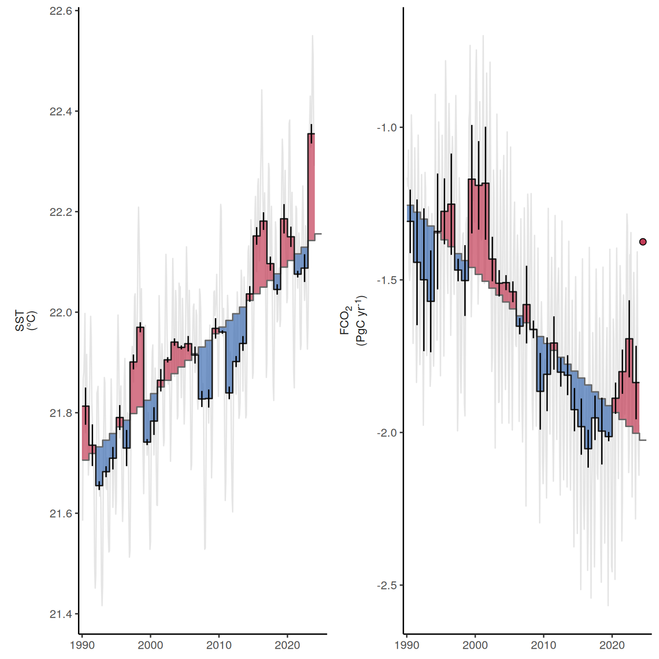
| Version | Author | Date |
|---|---|---|
| 265b0a8 | jens-daniel-mueller | 2025-06-06 |
ggsave(width = 10,
       height = 2,
       dpi = 1200,
       filename = "../output/timeseries_ensemble_mean_pco2_products_presentation_2024.pdf")

bind_rows(
  pco2_product_biome_annual_anomaly,
  pco2_product_biome_annual_anomaly %>%
    filter(year == max(year)) %>%
    mutate(year = year + 1) %>%
    select(-c(resid))
) %>%
  filter(name %in% c("fgco2_int", "temperature"),
         biome == "Global non-polar") %>%
  ggplot() +
  geom_path(
    data = pco2_product_biome_monthly_anomaly %>%
      filter(name %in% c("fgco2_int", "temperature"),
             biome == "Global non-polar"),
    aes(year + month / 12, value),
    col = "grey90"
  )+
  geom_rect(
    data = . %>% filter(year != max(year)),
    aes(
      xmin = year,
      xmax = year + 1,
      ymin = fit,
      ymax = value,
      fill = as.factor(sign(-resid))
    ),
    alpha = 0.5
  ) +
  geom_step(aes(year, fit, col = "Baseline")) +
  geom_step(aes(year, value, col = "Observed")) +
  scale_color_manual(values = c("grey40", "grey10"),
                     name = "Annual means") +
  scale_fill_manual(
    values = c(warm_color, cold_color),
    labels = c("positive", "negative"),
    name = "Anomalies"
  ) +
  guides(
    color = guide_legend(order = 1),
    fill = guide_legend(order = 2)
  ) +
  scale_x_continuous(limits = c(1989.5,2024.5), expand = c(0,0),
                     breaks = c(1990,2010)) +
  facet_grid(
    name ~ product,
    scales = "free_y",
    labeller = labeller(name = x_axis_labels),
    switch = "y"
  ) +
  theme(
    axis.title = element_blank(),
    strip.text.y.left = element_markdown(),
    strip.placement = "outside",
    strip.background.y = element_blank(),
    legend.position = "none",
    legend.direction = "vertical"
  )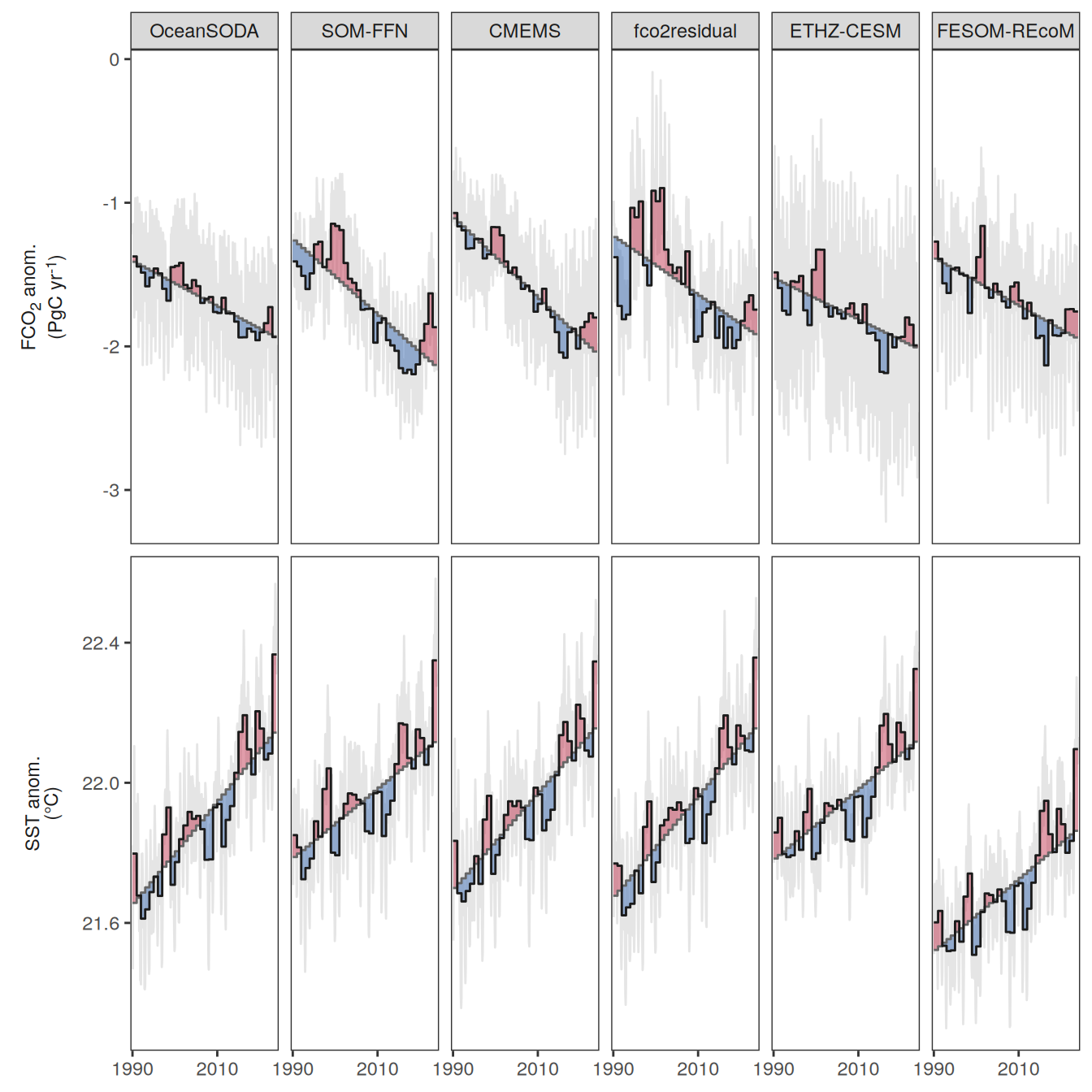
| Version | Author | Date |
|---|---|---|
| 265b0a8 | jens-daniel-mueller | 2025-06-06 |
ggsave(width = 8,
       height = 3,
       dpi = 600,
       filename = "../output/timeseries_all_products.pdf")


bind_rows(
  pco2_product_biome_monthly_anomaly,
  pco2_product_biome_monthly_anomaly %>%
    filter(year == max(year),
           month == 12) %>%
    mutate(month = month + 1)
) %>%
  mutate(year = year + month/12) %>%
  filter(name %in% c("fgco2_int", "temperature"),
         product == if(GCB_products){"OceanSODA"}else{"OceanSODAv2"},
         biome == "Global non-polar",
         year >= 2010) %>%
  ggplot() +
  geom_rect(
    data = . %>% filter(year != max(year)),
    aes(
      xmin = year,
      xmax = year + 1/12,
      ymin = fit,
      ymax = value,
      fill = as.factor(sign(-resid))
    ),
    alpha = 0.5
  ) +
  geom_step(aes(year, fit, col = "Baseline")) +
  scale_color_manual(values = c("grey40", "grey10"),
                     name = "Annual means") +
  scale_fill_manual(
    values = c(warm_color, cold_color),
    labels = c("positive", "negative"),
    name = "Anomalies"
  ) +
  guides(color = guide_legend(order = 1),
         fill = guide_legend(order = 2))+
  facet_grid(
    name ~ .,
    scales = "free_y",
    labeller = labeller(name = x_axis_labels),
    switch = "y"
  ) +
  coord_cartesian(expand = 0) +
  theme(
    axis.title = element_blank(),
    strip.text.y.left = element_markdown(),
    strip.placement = "outside",
    strip.background.y = element_blank(),
    legend.position = "top",
    legend.direction = "vertical"
  )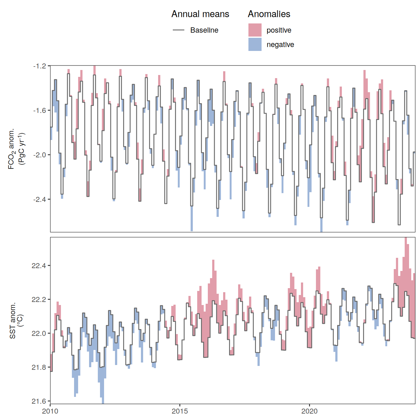
| Version | Author | Date |
|---|---|---|
| 265b0a8 | jens-daniel-mueller | 2025-06-06 |
SOM_FFN_biome_annual_anomaly <-
  bind_rows(
    pco2_product_biome_annual_anomaly %>%
      filter(
        name %in% c("fgco2_int", "temperature"),
        biome == "Global non-polar",
        product %in% "SOM-FFN"
      ) %>%
      select(-product) %>%
      mutate(year_anom = "2023"),
    SOM_FFN_predict_2024_biome_annual_anomaly %>%
      filter(
        name %in% c("fgco2_int", "temperature"),
        biome == "Global non-polar"
      ) %>%
      mutate(year_anom = "2024")
  )

p_value <- SOM_FFN_biome_annual_anomaly %>%
  ggplot(aes(year, value, col = year_anom)) +
  geom_path() +
  facet_wrap(
    . ~ name,
    scales = "free_y",
    strip.position = "left",
    labeller = labeller(name = x_axis_labels_abs)
  )+
  labs(x = "Year") +
  scale_color_okabeito() +
  theme(
    axis.title.y = element_blank(),
    axis.title.x = element_blank(),
    strip.text.y.left = element_markdown(),
    strip.placement = "outside",
    strip.background.y = element_blank(),
    legend.title = element_blank()
  )

p_resid <- SOM_FFN_biome_annual_anomaly %>%
  ggplot(aes(year, resid, col = year_anom)) +
  geom_hline(yintercept = 0, col = "grey") +
  geom_path() +
  facet_wrap(
    . ~ name,
    scales = "free_y",
    strip.position = "left",
    labeller = labeller(name = x_axis_labels)
  )+
  labs(x = "Year") +
  scale_color_okabeito() +
  theme(
    axis.title.y = element_blank(),
    axis.title.x = element_blank(),
    strip.text.y.left = element_markdown(),
    strip.placement = "outside",
    strip.background.y = element_blank(),
    legend.title = element_blank()
  )

p_value / p_resid

ggsave(width = 8,
       height = 4,
       dpi = 600,
       filename = "../output/timeseries_flux_sst_SOM-FFN.pdf")

SOM_FFN_biome_annual_anomaly %>%
  select(name, resid, year_anom, year) %>%
  pivot_wider(values_from = resid) %>%
  ggplot(aes(temperature, fgco2_int)) +
  geom_point() +
  geom_smooth(method = "lm") +
  facet_wrap(~ year_anom)


lm_fgco2_sst <- SOM_FFN_biome_annual_anomaly %>%
  select(year, year_anom, name, resid) %>%
  pivot_wider(values_from = resid) %>%
  nest(data = -year_anom) %>%
  mutate(fit = map(data, ~ lm(
    formula = fgco2_int ~ temperature,
    data = .x %>% filter(year < 2023)
  )))

# predict fgco2 anomaly from SST anomaly per biome
# include anomaly year for prediction

lm_fgco2_sst <- lm_fgco2_sst %>%
  mutate(resid = map2(fit, data, predict)) %>%
  unnest(c(data, resid))


# compute unexpected (predicted vs observed) flux anomalies

lm_fgco2_sst %>%
  select(year, year_anom, fgco2_int, resid) %>%
  pivot_longer(c(fgco2_int, resid)) %>%
  ggplot(aes(year, value, col = year_anom)) +
  geom_hline(yintercept = 0) +
  geom_path() +
  facet_wrap(~ name) +
  scale_color_okabeito() +
  labs(title = "Unexpected residuals in ocean carbon sink",
       subtitle = "Linear regression baseline + global mean SST anomaly") +
  theme(legend.title = element_blank(),
        axis.title.x = element_blank())

lm_fgco2_sst %>%
  ggplot(aes(year, fgco2_int-resid, col = year_anom)) +
  geom_hline(yintercept = 0) +
  geom_path() +
  scale_color_okabeito() +
  labs(title = "Unexpected residuals in ocean carbon sink",
       subtitle = "Linear regression baseline + global mean SST anomaly",
       y = paste("Unexpected", labels_breaks("fgco2_int")$i_legend_title)) +
  theme(legend.title = element_blank(),
        axis.title.x = element_blank(),
        axis.title.y = element_markdown())


ggsave(width = 8,
       height = 4,
       dpi = 600,
       filename = "../output/timeseries_flux_anomaly_SOM-FFN.pdf")

# SOM_FFN_biome_annual_anomaly_lm_fgco2_sst <-
#   inner_join(
#     SOM_FFN_biome_annual_anomaly %>%
#       filter(
#         name %in% c("fgco2_int")
#       ) %>%
#       select(year, year_anom, baseline = fit),
#     lm_fgco2_sst %>%
#       select(year, year_anom, resid)
#   )
#
#
# lm_fgco2_sst <-
#   lm_fgco2_sst %>%
#   mutate(unexplained = fgco2_int - resid)
#
#
# lm_fgco2_sst %>%
#   ggplot(aes(year, unexplained, col = year_anom)) +
#   geom_hline(yintercept = 0) +
#   geom_path() +
#   labs(title = "Unexpected residuals in ocean carbon sink",
#        subtitle = "Linear regression baseline + global mean SST anomaly")
df_baseline <-
pco2_product_biome_annual_anomaly %>%
filter(biome == "Global non-polar",
name %in% c("fgco2_int", "temperature"),
product %in% pco2_product_list) %>%
select(product, year, name, value) %>%
pivot_wider() %>%
rename(fgco2_int_observed = fgco2_int)
df_baseline <-
inner_join(df_baseline, co2_annmean_gl %>% select(year, atmco2 = mean))
df_baseline <-
inner_join(df_baseline, co2_gr_gl %>% select(year, atmco2_gr = `ann inc`))
df_baseline <-
inner_join(df_baseline, nino_sst %>%
group_by(year) %>%
summarise(nino34 = mean(resid)) %>%
ungroup())
df_baseline <-
inner_join(
df_baseline,
pco2_product_biome_annual_anomaly_lm_fgco2_sst %>%
mutate(fgco2_int_predict_baseline_global_SST = baseline + resid) %>%
select(product, year, fgco2_int_predict_baseline_global_SST)
)
df_baseline %>%
pivot_longer(-c(year, product)) %>%
ggplot(aes(year, value)) +
geom_path() +
facet_grid(name ~ product, scales = "free_y")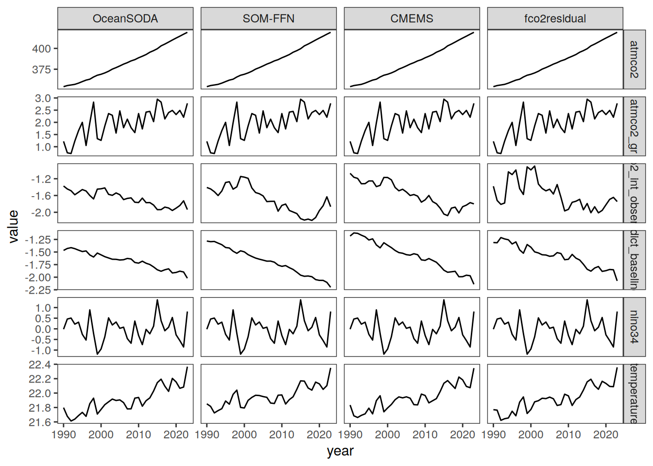
df_baseline %>%
  select(-fgco2_int_predict_baseline_global_SST) %>%
  pivot_longer(-c(product, year, fgco2_int_observed)) %>%
  ggplot(aes(value, fgco2_int_observed)) +
  geom_path(col = "grey80") +
  geom_point(aes(fill = year),
             shape = 21) +
  scale_fill_viridis_c() +
  facet_grid(product ~ name, scales = "free")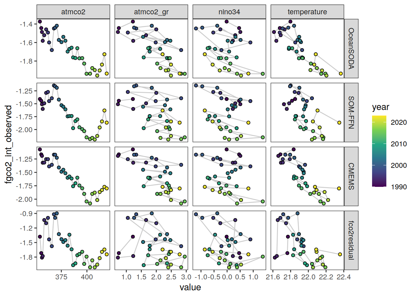
# fit lin. reg. model fgco2 anomaly vs SST anomaly per biome
# excluding anomaly year from fit

mlr <- df_baseline %>%
  nest(data = -product) %>%
  mutate(fit = map(data, ~ lm(
    formula = fgco2_int_observed ~ atmco2 + atmco2_gr + nino34,
    data = .x %>% filter(year != 2023)
  )))

# predict fgco2 anomaly from SST anomaly per biome
# include anomaly year for prediction

mlr <- mlr %>%
  mutate(fgco2_int_predict_atm_nino = map2(fit, data, predict)) %>%
  unnest(c(data, fgco2_int_predict_atm_nino))

mlr %>%
  select(product, year, starts_with("fgco2_int")) %>%
  pivot_longer(starts_with("fgco2_int"),
               names_prefix = "fgco2_int_") %>%
  ggplot(aes(year, value, col = name)) +
  geom_path() +
  geom_smooth(data = . %>% filter(name == "observed",
                                  year != 2023),
              method = "lm",
              se = FALSE,
              fullrange = TRUE) +
  scale_color_okabeito() +
  facet_wrap(~ product) +
  labs(y = str_remove(labels_breaks("fgco2_int")$i_legend_title, "anom.")) +
  theme(axis.title.x = element_blank(),
        axis.title.y = element_markdown(),
        legend.title = element_blank())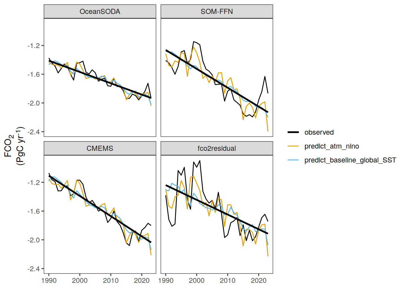
ggsave(width = 8,
       height = 4,
       dpi = 600,
       filename = "../output/timeseries_pco2_products_predictions.pdf")


mlr %>%
  mutate(
    unexpected_baseline_global_SST =
      fgco2_int_observed - fgco2_int_predict_baseline_global_SST,
    unexpected_atm_nino =
      fgco2_int_observed - fgco2_int_predict_atm_nino,
  ) %>%
  select(product, year, starts_with("unex")) %>%
  pivot_longer(starts_with("unex"),
               names_prefix = "unexpected_") %>%
  ggplot(aes(year, value, col = name)) +
  geom_hline(yintercept = 0) +
  geom_path() +
  scale_color_okabeito() +
  facet_wrap(~ product) +
  labs(y = labels_breaks("fgco2_int")$i_legend_title) +
  theme(axis.title.x = element_blank(),
        axis.title.y = element_markdown(),
        legend.title = element_blank())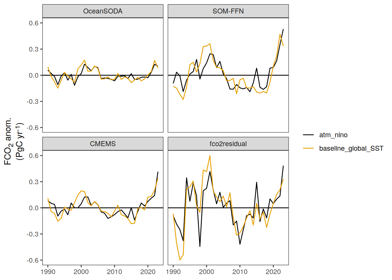
| Version | Author | Date |
|---|---|---|
| b031240 | jens-daniel-mueller | 2025-03-11 |
mlr_ensemble <- mlr %>%
  mutate(
    unexpected_baseline_global_SST =
      fgco2_int_observed - fgco2_int_predict_baseline_global_SST,
    unexpected_atm_nino =
      fgco2_int_observed - fgco2_int_predict_atm_nino,
  ) %>%
  select(product, year, starts_with("unex")) %>%
  pivot_longer(starts_with("unex"), names_prefix = "unexpected_") %>%
  group_by(year, name) %>%
  summarise(sd = sd(value),
            value = mean(value)) %>%
  ungroup()

mlr_ensemble %>%
  mutate(name = case_when(
    name == "atm_nino" ~ "Multiple linear regression",
    name == "baseline_global_SST" ~ "Linear baseline + global mean SST",
  )) %>%
  ggplot(aes(year, value,
             ymin = value - sd,
             ymax = value + sd)) +
  geom_hline(yintercept = 0) +
  geom_ribbon(alpha = 0.2) +
  geom_path() +
  scale_color_okabeito() +
  facet_wrap(~ name) +
  labs(y = paste("Unexpected", labels_breaks("fgco2_int")$i_legend_title)) +
  theme(axis.title.x = element_blank(),
        axis.title.y = element_markdown(),
        legend.title = element_blank())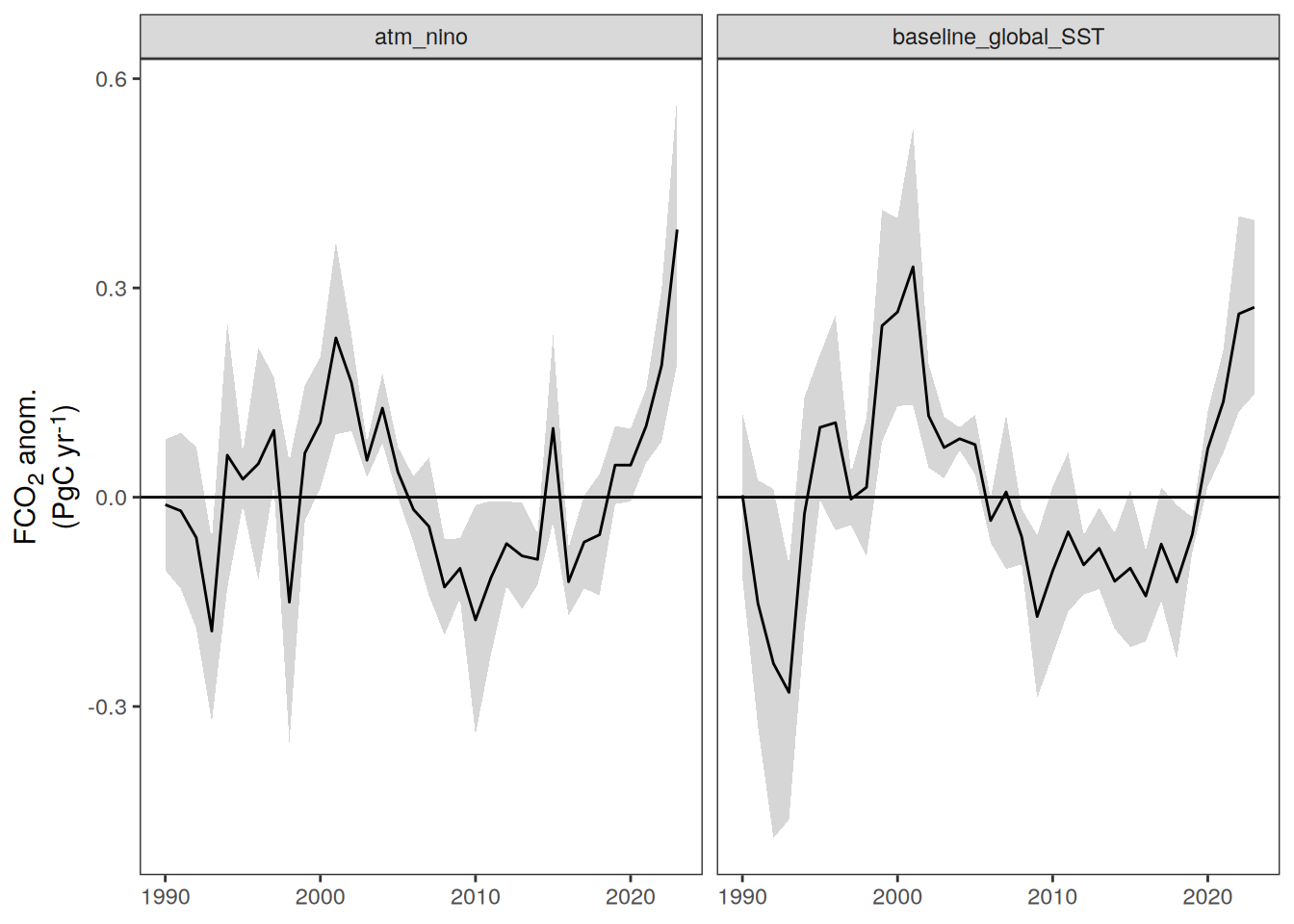
ggsave(width = 7,
       height = 3,
       dpi = 600,
       filename = "../output/timeseries_pco2_products_predictions_ensemble_mean.pdf")

mlr_ensemble %>%
  filter(year == 2023)
# A tibble: 2 × 4
year name sd value
<dbl> <chr> <dbl> <dbl>
1 2023 atm_nino 0.192 0.384
2 2023 baseline_global_SST 0.125 0.272pco2_product_biome_annual_anomaly %>%
filter(year == 2023,
name %in% c("fgco2", "fgco2_int", "dfco2",
"kw_sol", "temperature",
"no3", "mld", "intpp", "chl")) %>%
mutate(region = case_when(biome == "Global non-polar" ~ "Global non-polar",
# biome %in% super_biomes ~ "Super biomes",
TRUE ~ "Biomes"),
region = factor(region, levels = c("Global non-polar", "Biomes"))) %>%
group_split(name) %>%
# head(1) %>%
map(
~ ggplot(data = .x) +
geom_col(aes(biome, value, fill = product),
position = "dodge2") +
scale_fill_manual(values = color_products) +
geom_col(aes(biome, fit, group = product, col = paste0(2023,"\nlinear\nprediction")),
position = "dodge2",
fill = "transparent") +
labs(y = labels_breaks(unique(.x$name))$i_legend_title,
title = "Absolute") +
scale_color_grey() +
facet_grid(.~region, scales = "free_x", space = "free_x") +
theme(legend.title = element_blank(),
axis.text.x = element_text(angle = 90, vjust = 0.5, hjust=1),
axis.title.x = element_blank(),
axis.title.y = element_markdown(),
strip.background = element_blank(),
legend.position = "top")
)[[1]]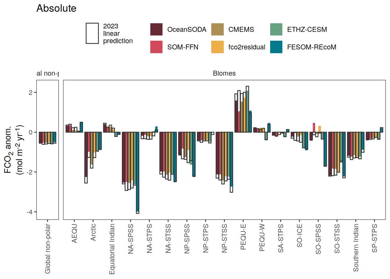
[[2]]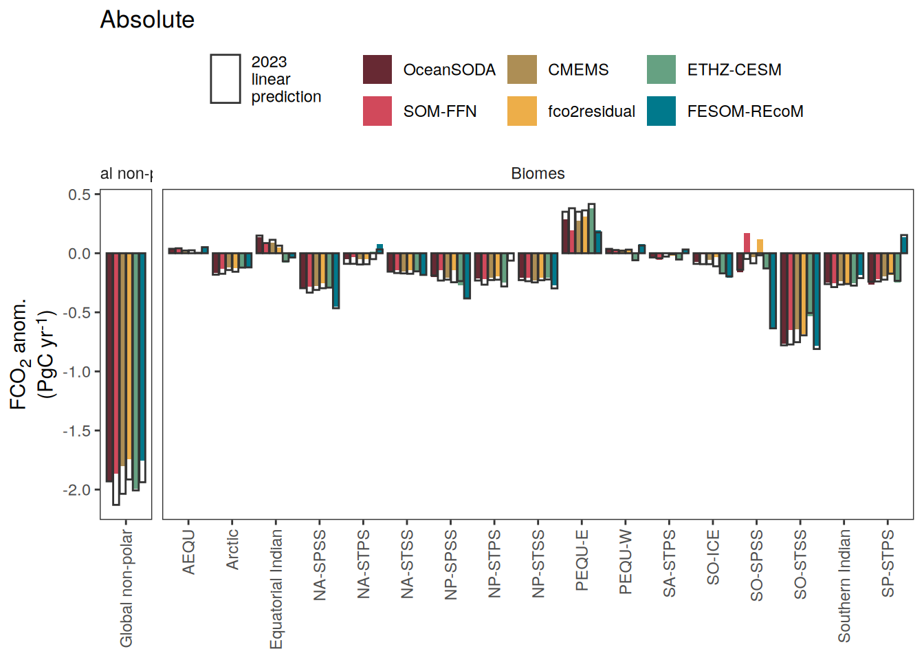
[[3]]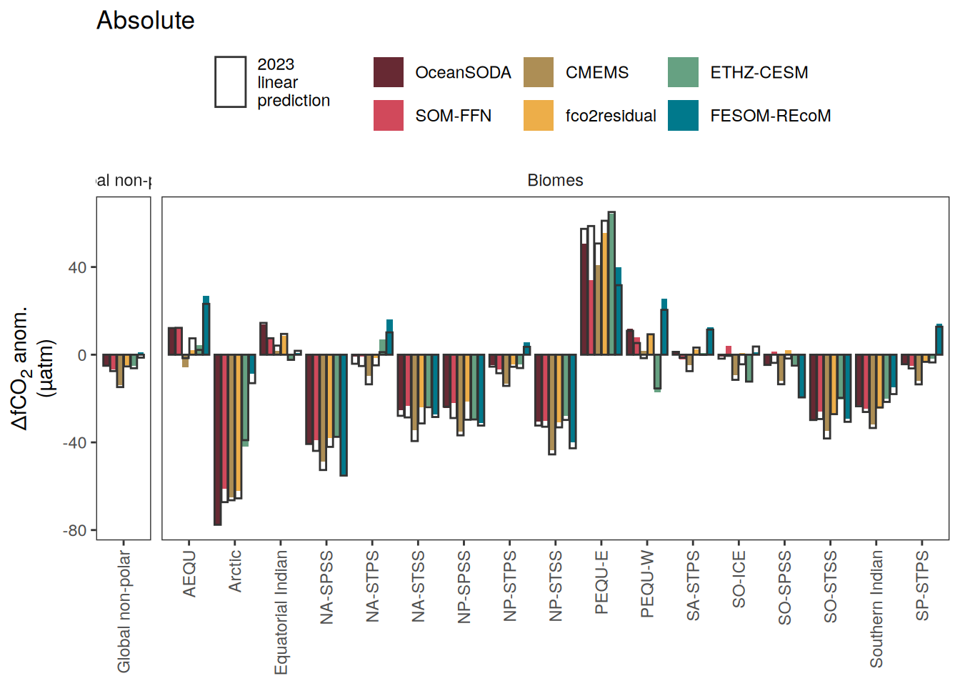
[[4]]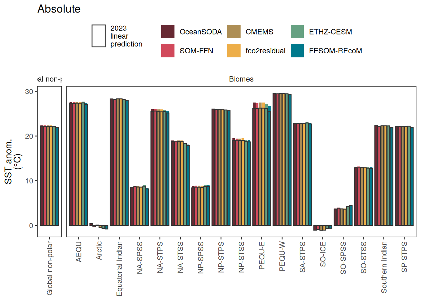
[[5]]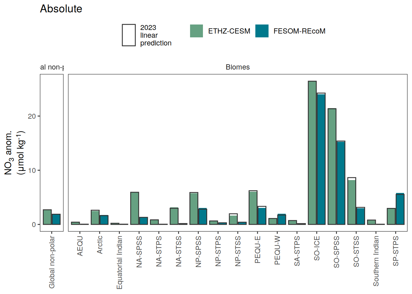
| Version | Author | Date |
|---|---|---|
| 518e3d0 | jens-daniel-mueller | 2025-02-27 |
[[6]]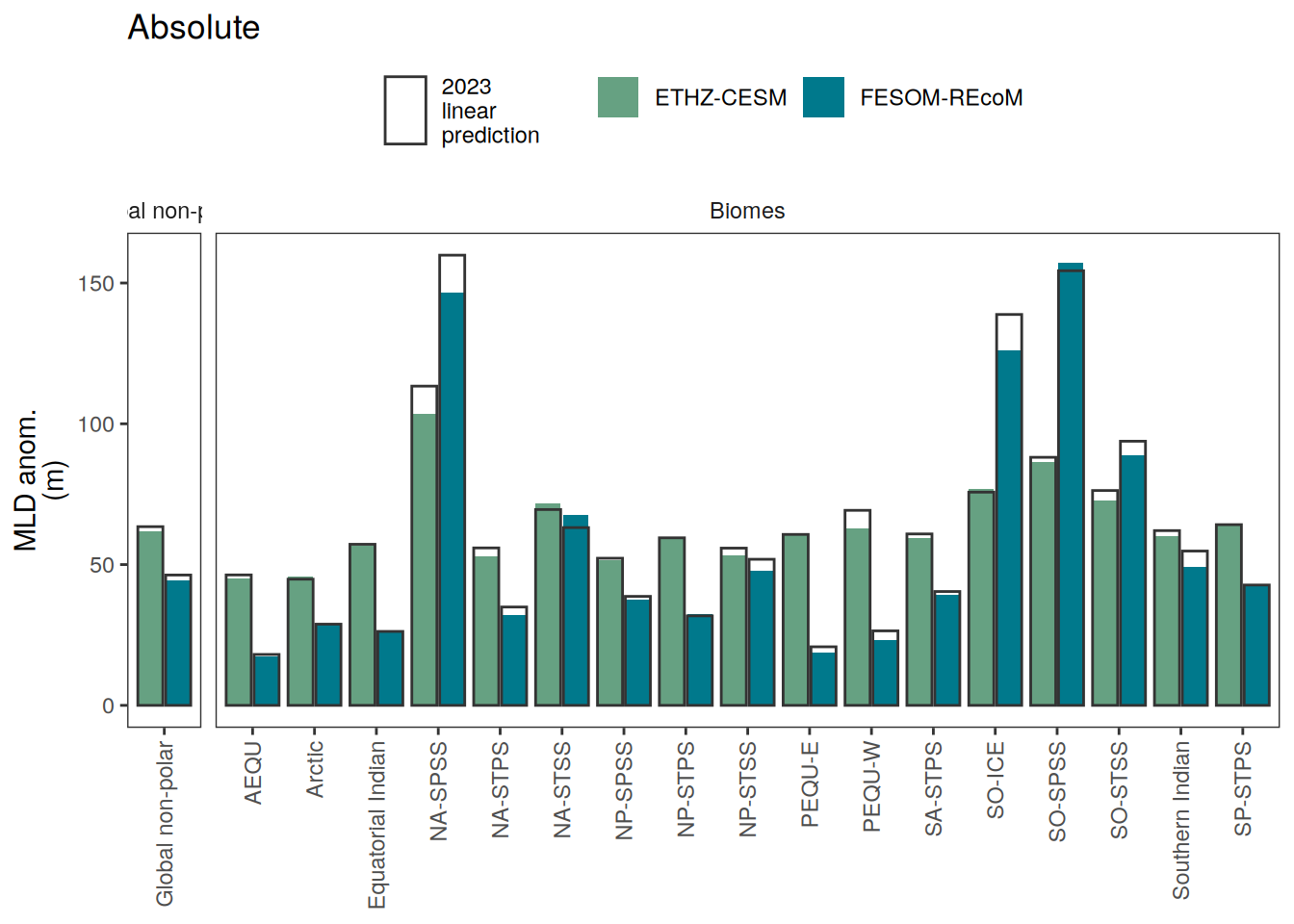
| Version | Author | Date |
|---|---|---|
| 518e3d0 | jens-daniel-mueller | 2025-02-27 |
[[7]]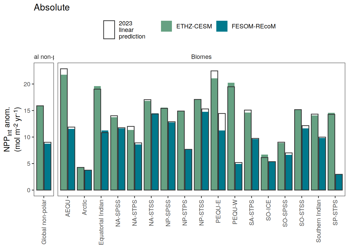
| Version | Author | Date |
|---|---|---|
| 518e3d0 | jens-daniel-mueller | 2025-02-27 |
[[8]]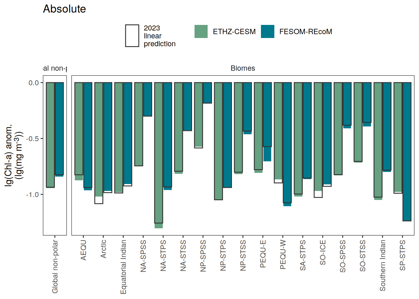
| Version | Author | Date |
|---|---|---|
| 518e3d0 | jens-daniel-mueller | 2025-02-27 |
full_join(
  pco2_product_biome_annual_anomaly %>%
    filter(year != 2023,
           name %in% name_core) %>%
    group_by(product, name, biome) %>%
    summarise(resid_sd = sd(resid)) %>%
    ungroup(),
  pco2_product_biome_annual_anomaly %>%
    filter(year == 2023,
           name %in% name_core)) %>%
  mutate(
    region = case_when(
      biome == "Global non-polar" ~ "Global non-polar",
      TRUE ~ "Biomes"
    ),
    region = factor(region, levels = c("Global non-polar", "Biomes"))
  ) %>%
  group_split(name) %>%
  # head(1) %>%
  map(
    ~ ggplot(data = .x) +
      geom_col(aes(biome, value - fit, fill = product),
                 position = "dodge2") +
      scale_fill_manual(values = color_products) +
      geom_col(aes(biome, resid_sd * sign(value - fit),
                   group = product, col = paste0("Anomaly SD\nexcl.",2023)),
               position = "dodge2",
               fill = "transparent") +
      labs(y = labels_breaks(unique(.x$name))$i_legend_title,
           title = "Anomalies") +
      scale_color_grey() +
      facet_grid(.~region, scales = "free_x", space = "free_x") +
      theme(legend.title = element_blank(),
            axis.text.x = element_text(angle = 90, vjust = 0.5, hjust=1),
            axis.title.x = element_blank(),
            axis.title.y = element_markdown(),
            strip.background = element_blank(),
            legend.position = "top")
  )
[[1]]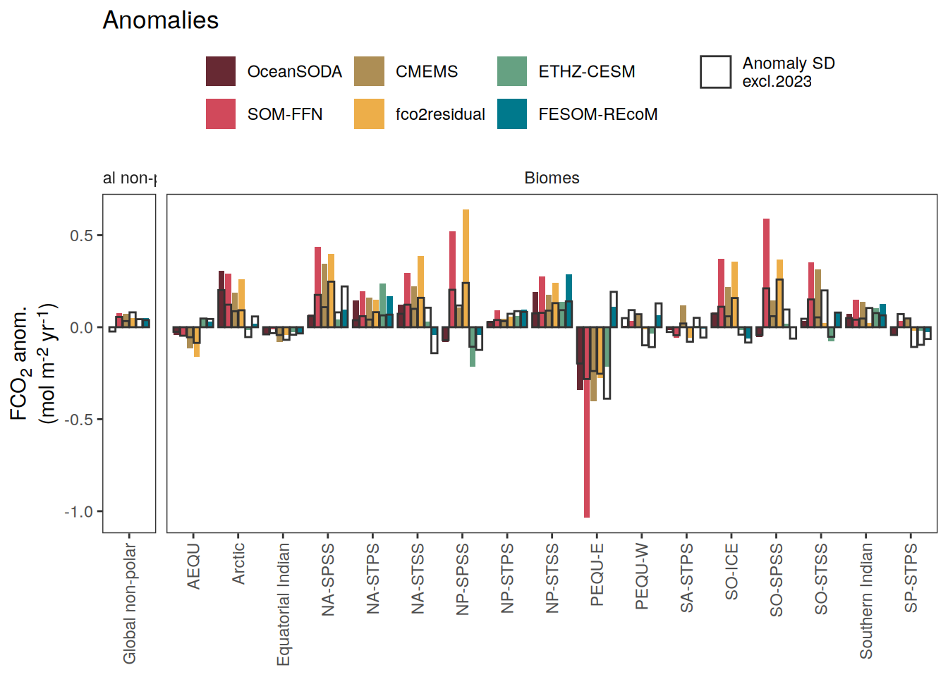
[[2]]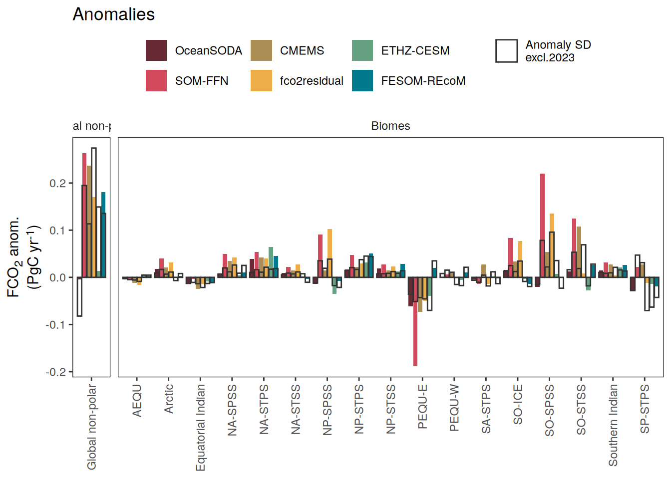
[[3]]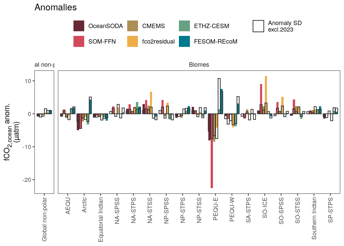
[[4]]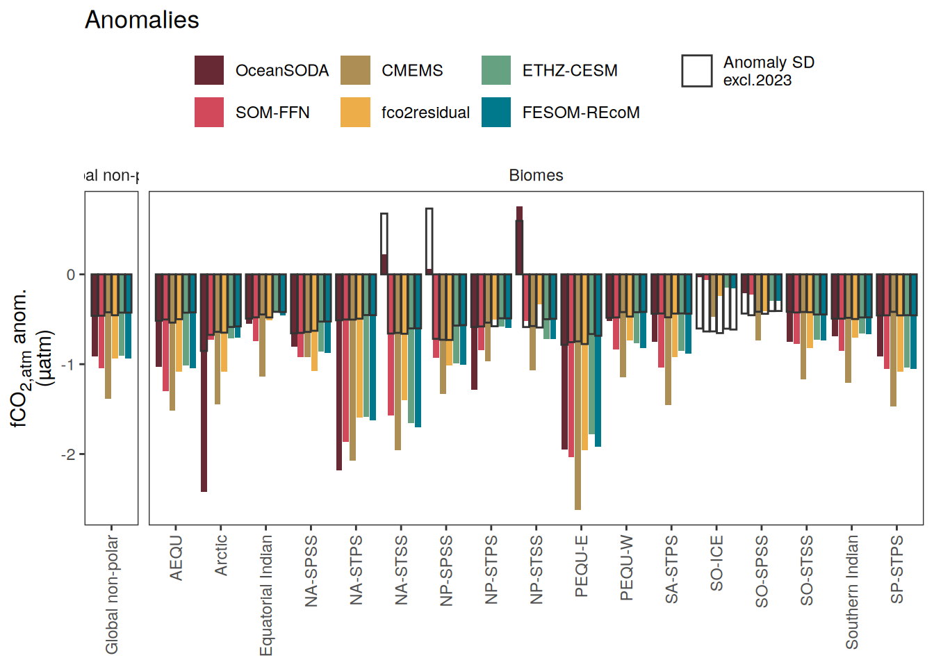
[[5]]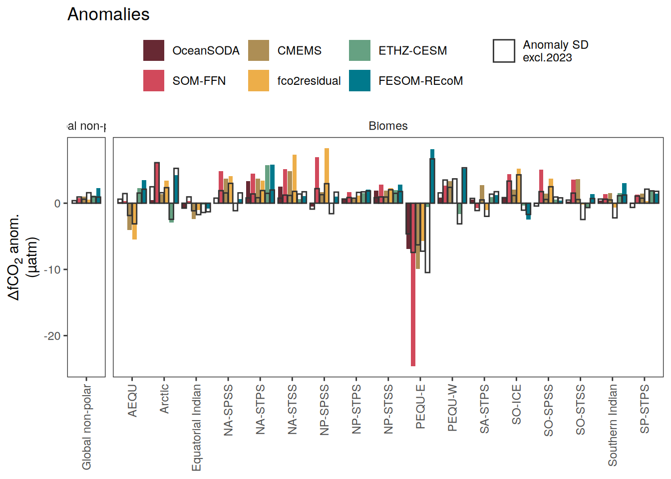
[[6]]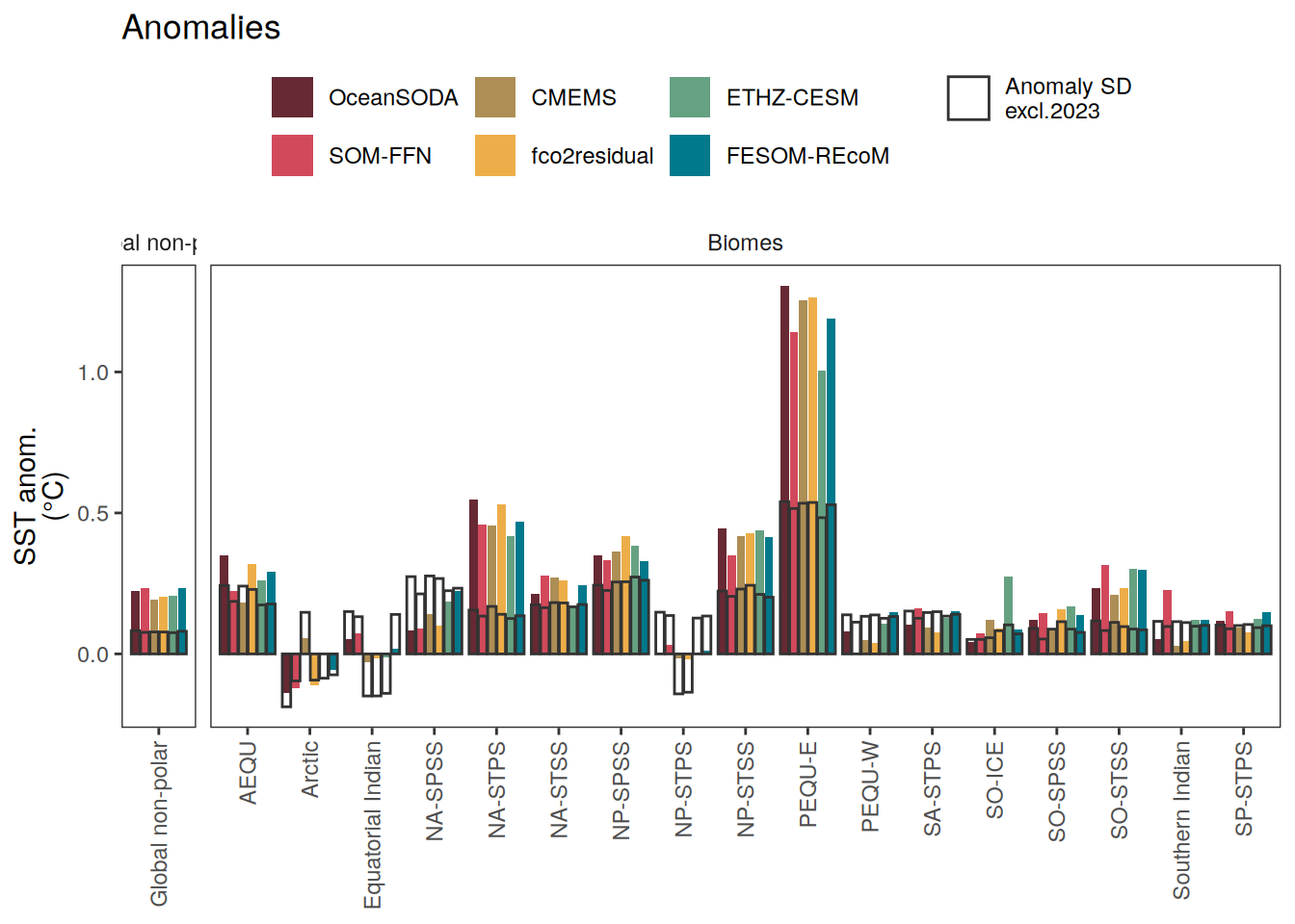
[[7]]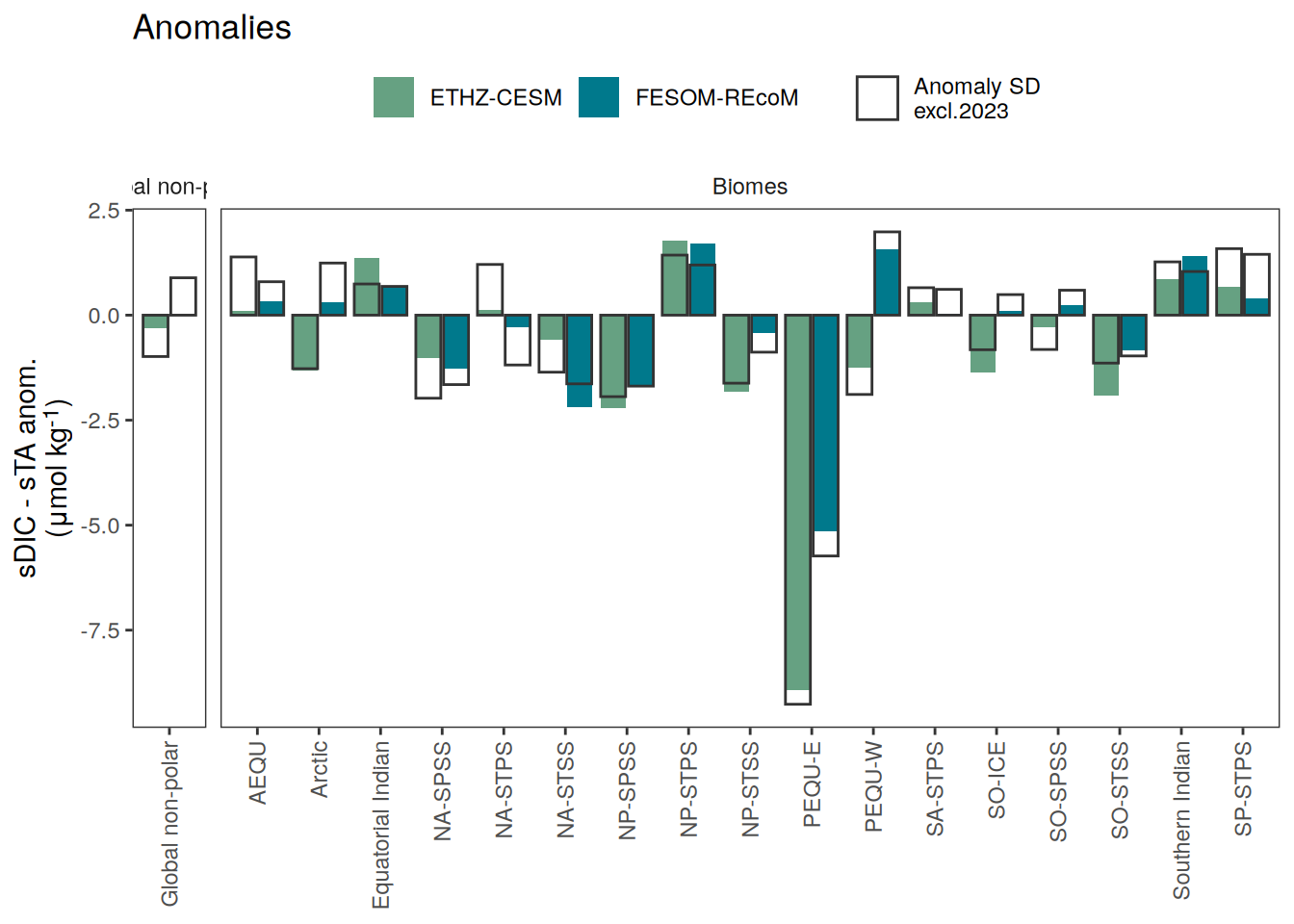
[[8]]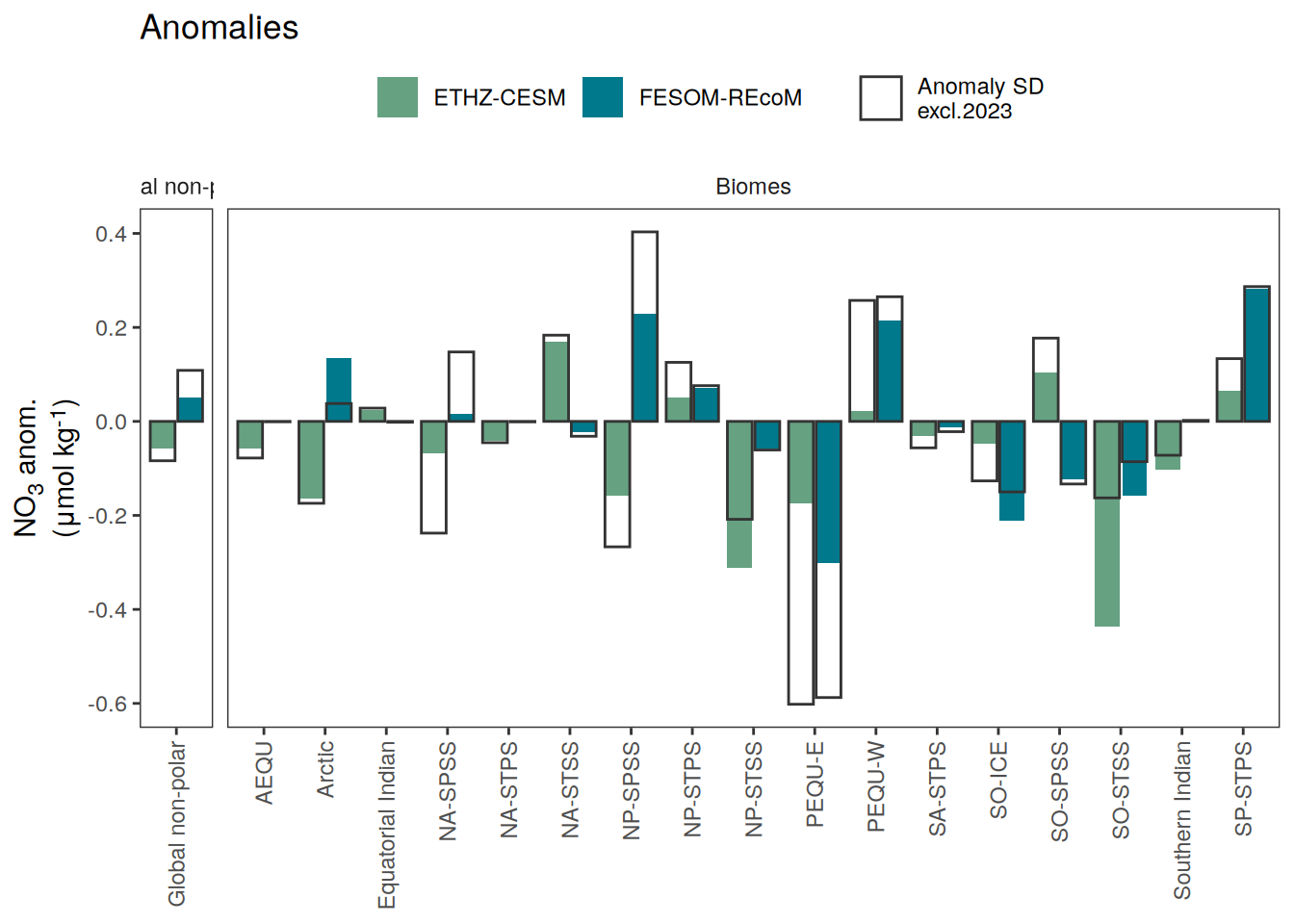
[[9]]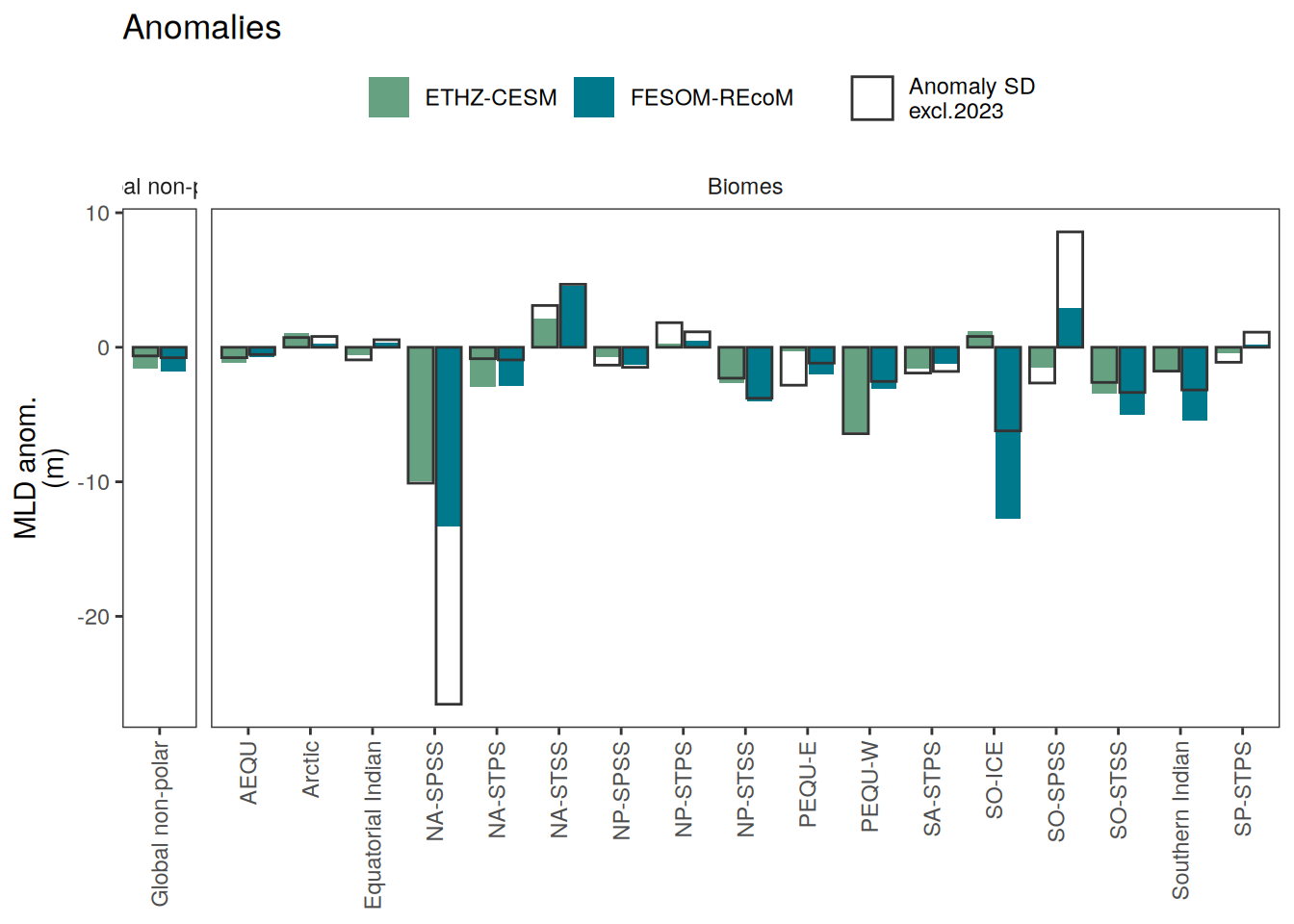
[[10]]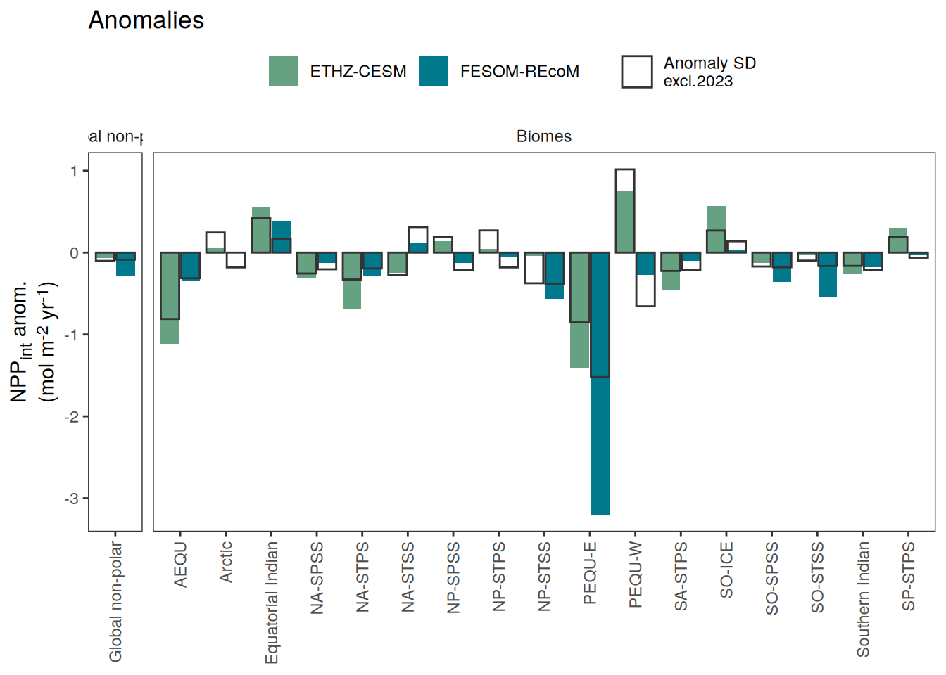
| Version | Author | Date |
|---|---|---|
| 1398df0 | jens-daniel-mueller | 2025-03-14 |
[[11]]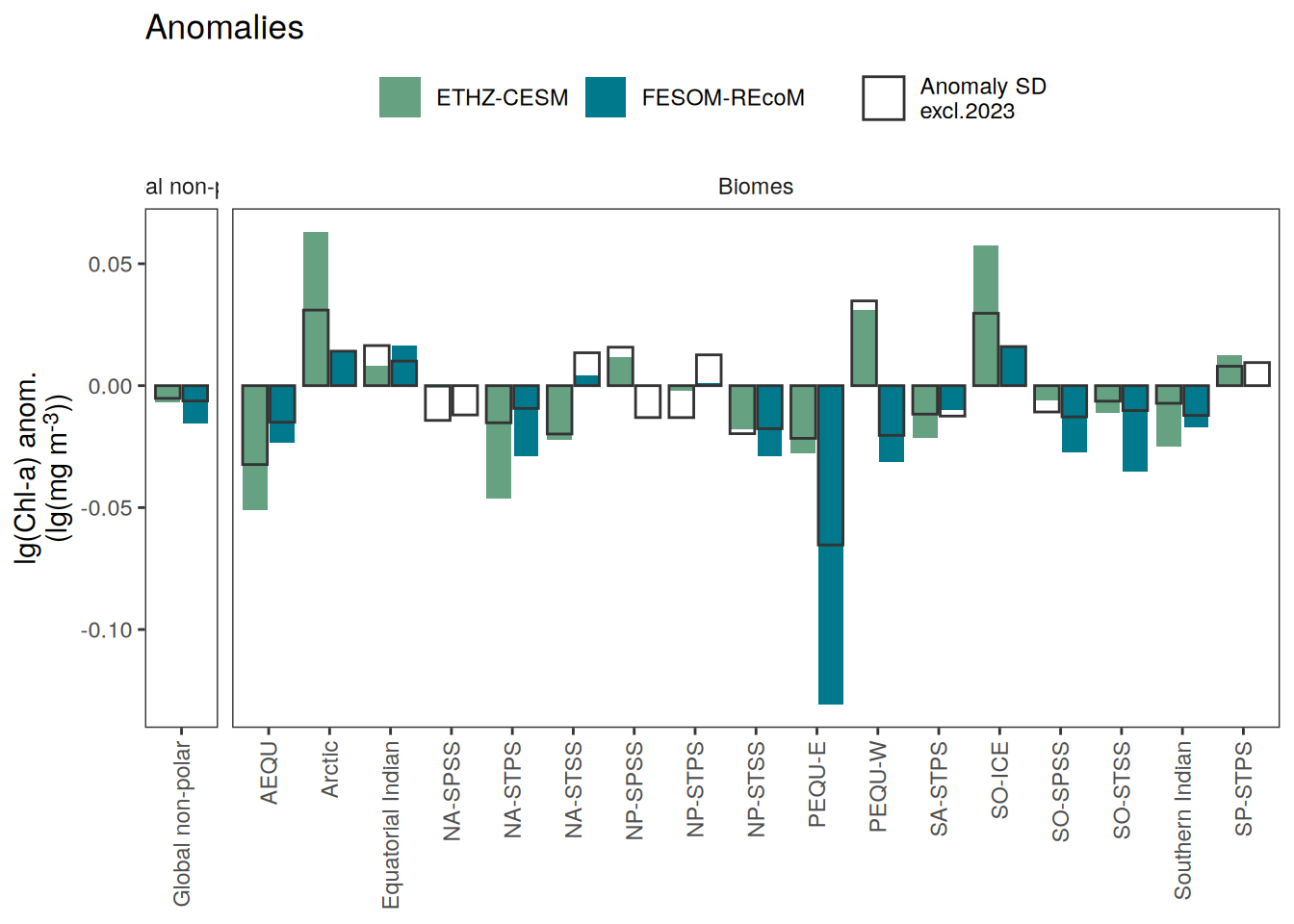
| Version | Author | Date |
|---|---|---|
| 1398df0 | jens-daniel-mueller | 2025-03-14 |
Super regions
pco2_product_biome_annual_anomaly_super_regions <-
  full_join(
    pco2_product_biome_annual_anomaly %>%
      filter(biome != "Global non-polar"),
    biome_mask %>%
      mutate(area = earth_surf(lat, lon)) %>%
      group_by(biome) %>%
      summarise(area = sum(area)) %>%
      ungroup()
  ) %>%
  pivot_longer(c(value,resid,fit),
               names_to = "estimate") %>%
  pivot_wider()

pco2_product_biome_annual_anomaly_super_regions <-
bind_rows(
  pco2_product_biome_annual_anomaly_super_regions %>%
    select(-biome) %>%
    group_by(product, estimate, year) %>%
    summarise(across(-c(fgco2_int, area),
                     ~ weighted.mean(., area, na.rm = TRUE)),
              across(fgco2_int,
                     ~ sum(., na.rm = TRUE))) %>%
    ungroup() %>%
    mutate(region = "Global"),
  pco2_product_biome_annual_anomaly_super_regions %>%
    filter(!str_detect(biome, "SO-ICE|SO-SPSS|Arctic")) %>%
    select(-biome) %>%
    group_by(product, estimate, year) %>%
    summarise(across(-c(fgco2_int, area),
                     ~ weighted.mean(., area, na.rm = TRUE)),
              across(fgco2_int,
                     ~ sum(., na.rm = TRUE))) %>%
    ungroup() %>%
    mutate(region = "Global non-polar"),
  pco2_product_biome_annual_anomaly_super_regions %>%
    filter(!str_detect(biome, "SO-ICE|Arctic")) %>%
    select(-biome) %>%
    group_by(product, estimate, year) %>%
    summarise(across(-c(fgco2_int, area),
                     ~ weighted.mean(., area, na.rm = TRUE)),
              across(fgco2_int,
                     ~ sum(., na.rm = TRUE))) %>%
    ungroup() %>%
    mutate(region = "Global ice-free"),
  pco2_product_biome_annual_anomaly_super_regions %>%
    filter(str_detect(biome, "NA-|NP-")) %>%
    select(-biome) %>%
    group_by(product, estimate, year) %>%
    summarise(across(-c(fgco2_int, area),
                     ~ weighted.mean(., area, na.rm = TRUE)),
              across(fgco2_int,
                     ~ sum(., na.rm = TRUE))) %>%
    ungroup() %>%
    mutate(region = "NH extratropics"),
  pco2_product_biome_annual_anomaly_super_regions %>%
    filter(str_detect(biome, "NA-")) %>%
    select(-biome) %>%
    group_by(product, estimate, year) %>%
    summarise(across(-c(fgco2_int, area),
                     ~ weighted.mean(., area, na.rm = TRUE)),
              across(fgco2_int,
                     ~ sum(., na.rm = TRUE))) %>%
    ungroup() %>%
    mutate(region = "North Atlantic"),
  pco2_product_biome_annual_anomaly_super_regions %>%
    filter(str_detect(biome, "NP-")) %>%
    select(-biome) %>%
    group_by(product, estimate, year) %>%
    summarise(across(-c(fgco2_int, area),
                     ~ weighted.mean(., area, na.rm = TRUE)),
              across(fgco2_int,
                     ~ sum(., na.rm = TRUE))) %>%
    ungroup() %>%
    mutate(region = "North Pacific"),
  pco2_product_biome_annual_anomaly_super_regions %>%
    filter(str_detect(biome, "PEQU|AEQU|Equ")) %>%
    select(-biome) %>%
    group_by(product, estimate, year) %>%
    summarise(across(-c(fgco2_int, area),
                     ~ weighted.mean(., area, na.rm = TRUE)),
              across(fgco2_int,
                     ~ sum(., na.rm = TRUE))) %>%
    ungroup() %>%
    mutate(region = "Tropics"),
  pco2_product_biome_annual_anomaly_super_regions %>%
    filter(str_detect(biome, "SA-|SP-|Southern|SO-STSS")) %>%
    select(-biome) %>%
    group_by(product, estimate, year) %>%
    summarise(across(-c(fgco2_int, area),
                     ~ weighted.mean(., area, na.rm = TRUE)),
              across(fgco2_int,
                     ~ sum(., na.rm = TRUE))) %>%
    ungroup() %>%
    mutate(region = "SH extratropics")) %>%
  mutate(region = fct_inorder(region)) %>%
  pivot_longer(-c(product, year, region, estimate)) %>%
  pivot_wider(names_from = estimate)

pco2_product_biome_annual_anomaly_super_regions %>%
  filter(year == 2023,
         name %in% c("fgco2", "fgco2_int", "dfco2", "temperature")) %>%
  group_split(name) %>%
  # head(1) %>%
  map(
    ~ ggplot(data = .x) +
      geom_hline(yintercept = 0) +
      geom_col(aes(region, value, fill = product),
                 position = "dodge2") +
      scale_fill_manual(values = color_products) +
      geom_col(aes(region, fit, group = product, col = paste0(2023,"\nlinear\nprediction")),
               position = "dodge2",
               fill = "transparent") +
      labs(y = str_remove(labels_breaks(unique(.x$name))$i_legend_title, " anom.")) +
      scale_color_grey() +
      facet_grid(.~region, scales = "free_x", space = "free_x") +
      theme(legend.title = element_blank(),
            axis.text.x = element_blank(),
            axis.title.x = element_blank(),
            axis.ticks.x = element_blank(),
            axis.title.y = element_markdown(),
            strip.background = element_blank(),
            legend.position = "top")
  )
[[1]]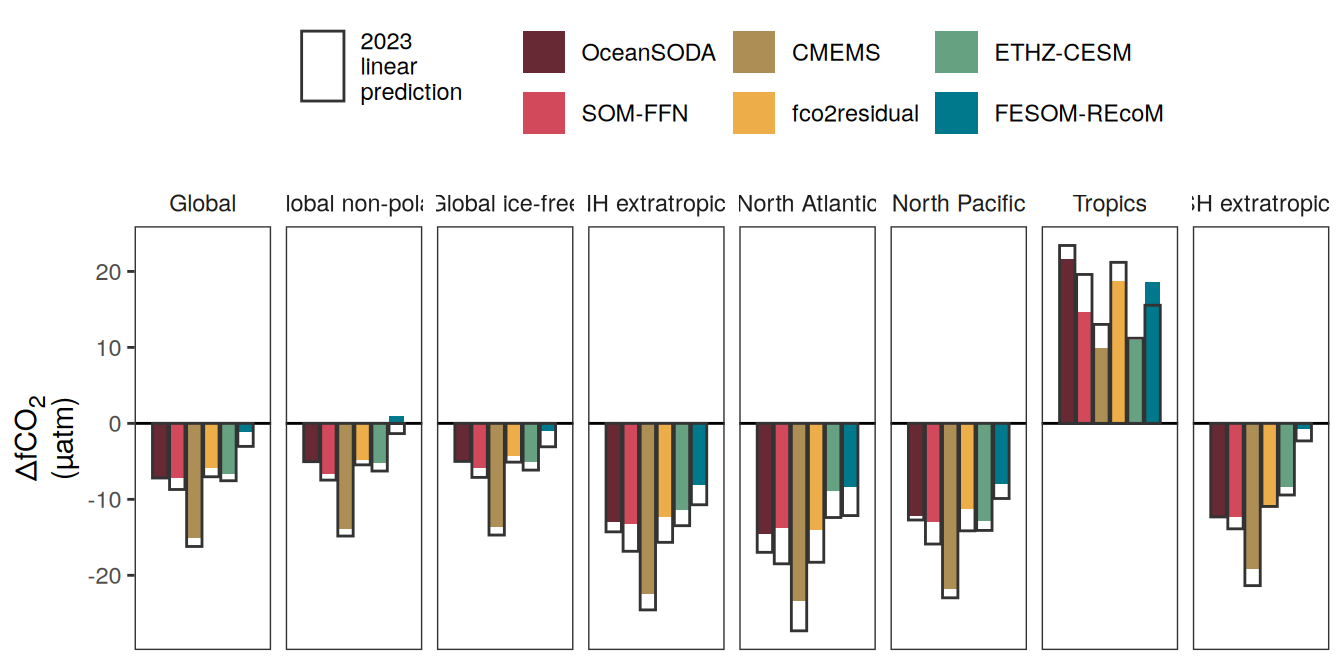
[[2]]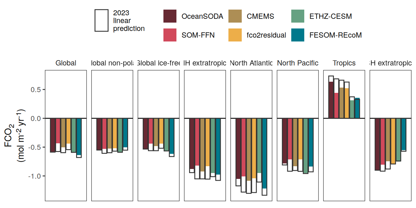
[[3]]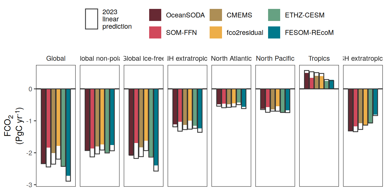
[[4]]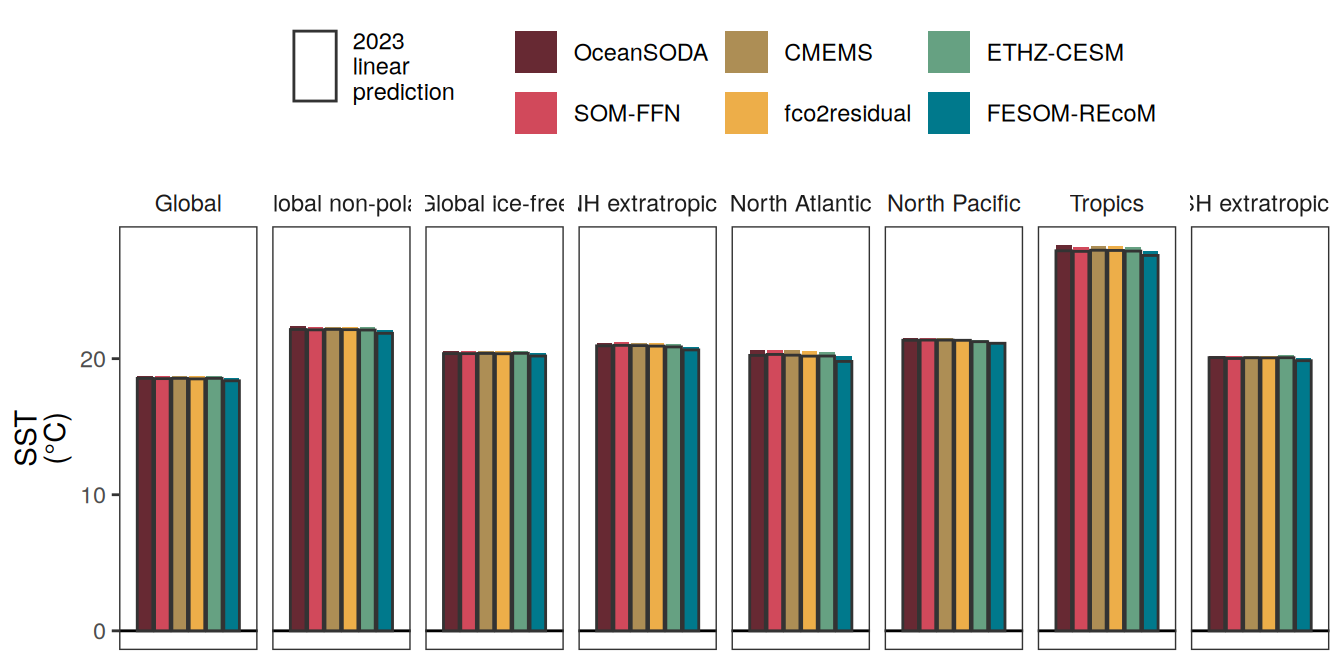
full_join(pco2_product_biome_annual_anomaly_super_regions %>%
  group_by(product, name, region) %>%
  summarise(resid_sd = sd(resid, na.rm = TRUE)) %>%
  ungroup(),
pco2_product_biome_annual_anomaly_super_regions %>%
  filter(year == 2023)) %>%
  filter(name %in% c("fgco2", "fgco2_int", "dfco2", "temperature")) %>%
  group_split(name) %>%
  # head(1) %>%
  map(
    ~ ggplot(data = .x) +
      geom_hline(yintercept = 0) +
      geom_col(aes(region, resid, fill = product),
               position = "dodge2") +
      scale_fill_manual(values = color_products) +
      geom_col(aes(region, resid_sd * sign(value - fit),
                   group = product, col = paste0("Anomaly SD\nexcl.",2023)),
               position = "dodge2",
               fill = "transparent") +
      labs(y = labels_breaks(unique(.x$name))$i_legend_title) +
      scale_color_grey() +
      facet_grid(. ~ region, scales = "free_x", space = "free_x") +
      theme(legend.title = element_blank(),
            axis.text.x = element_blank(),
            axis.title.x = element_blank(),
            axis.ticks.x = element_blank(),
            axis.title.y = element_markdown(),
            strip.background = element_blank(),
            legend.position = "top")
  )
[[1]]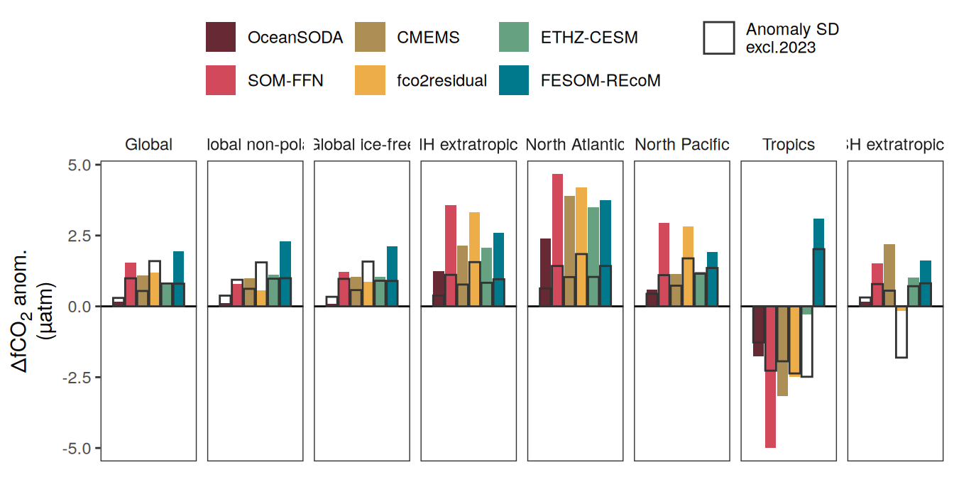
[[2]]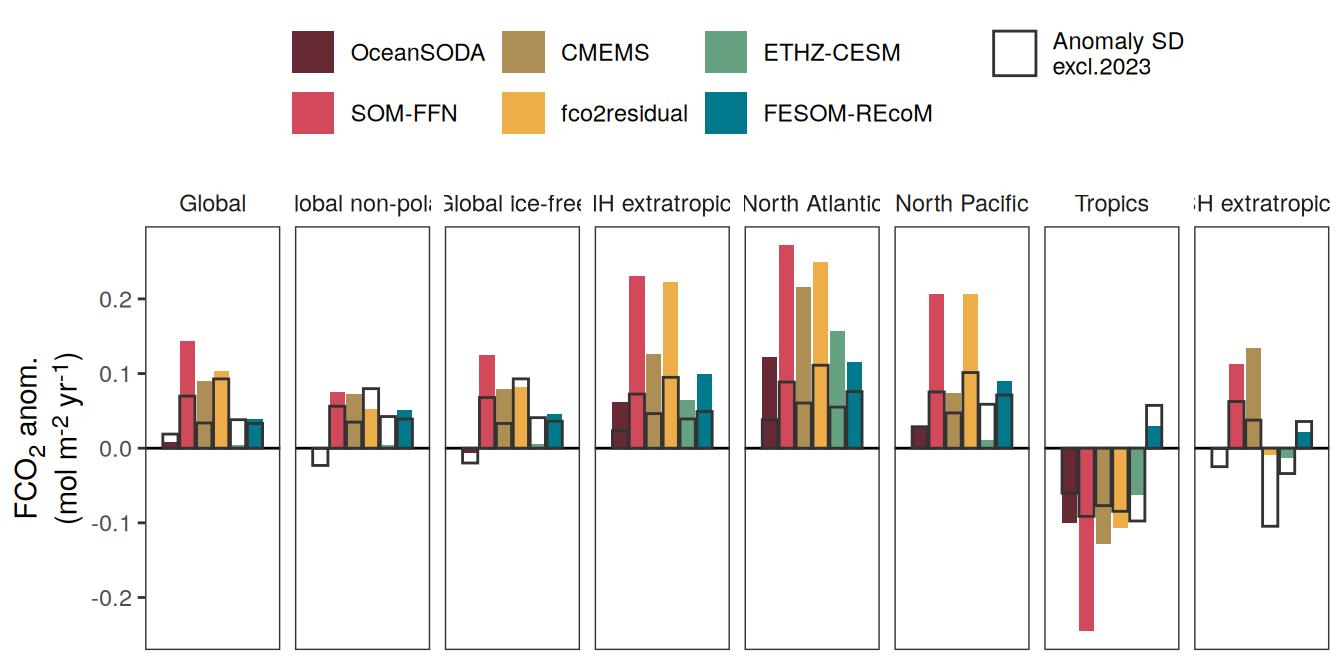
[[3]]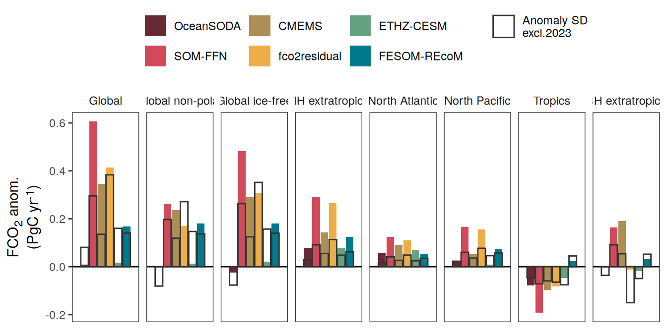
[[4]]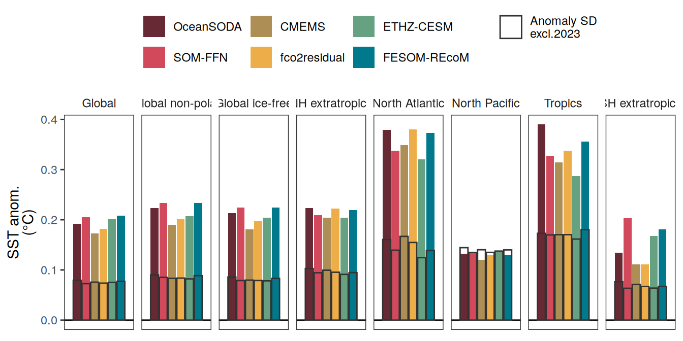
pco2_product_biome_annual_anomaly_super_regions <-
  bind_rows(
    pco2_product_biome_annual_anomaly_super_regions %>%
      filter(region != "Global ice-free") %>%
      rename(biome = region),
    pco2_product_biome_annual_anomaly %>%
      filter(biome != "Global non-polar")
  ) %>%
  filter(product %in% pco2_product_list) %>%
  group_by(year, name, biome) %>%
  summarise(
    resid_sd = sd(resid),
    resid = mean(resid),
    value_sd = sd(value),
    value = mean(value)
  ) %>%
  ungroup()


pco2_product_biome_annual_anomaly_super_regions <-
  pco2_product_biome_annual_anomaly_super_regions %>%
  filter(name %in% c("temperature", "fgco2", "fgco2_int"))

pco2_product_biome_annual_anomaly_super_regions %>%
  filter(year == 2023) %>%
  mutate(
    resid = paste(ifelse(
      resid > 0, paste0("+", format(round(resid, 2), nsmall = 2)), format(round(resid, 2), nsmall = 2)
    ), round(resid_sd, 2), sep = "±"),
    value = paste(ifelse(
      value > 0, paste0("+", format(round(value, 2), nsmall = 2)), format(round(value, 2), nsmall = 2)
    ), round(value_sd, 2), sep = "±"),
    resid = str_replace(resid, " ", ""),
    value = str_replace(value, " ", "")
  ) %>%
  select(-c(contains("_sd"), year)) %>%
  pivot_wider(values_from = c(resid, value)) %>%
  relocate(
    biome,
    value_temperature,
    resid_temperature,
    value_fgco2,
    resid_fgco2,
    value_fgco2_int,
    resid_fgco2_int
  ) %>%
  arrange(match(
    biome,
    c(
      "NA-SPSS",
      "NA-STSS",
      "NA-STPS",
      "North Atlantic",
      "NP-SPSS",
      "NP-STSS",
      "NP-STPS",
      "North Pacific",
      "NH extratropics",
      "PEQU-E",
      "PEQU-W",
      "AEQU",
      "Equatorial Indian",
      "Tropics",
      "SA-STPS",
      "SP-STPS",
      "Southern Indian",
      "SO-STSS",
      "SH extratropics",
      "Global non-polar",
      "SO-SPSS",
      "SO-ICE",
      "Arctic",
      "Global"
    )
  )) %>%
  write_csv("../output/biome_anomaly_ensemble_mean_pco2_products.csv")
pco2_product_biome_annual_anomaly_merged <-
full_join(region_biomes,
pco2_product_biome_annual_anomaly) %>%
mutate(region = case_when(biome == "Global non-polar" ~ "Global\nnon-polar",
region == "atlantic" ~ "Atlantic",
region == "pacific" ~ "Pacific",
region == "indian" ~ "Indian Ocean",
TRUE ~ region),
region = fct_rev(fct_inorder(region))) %>%
mutate(
latitude = case_when(
biome == "Global non-polar" ~ "Global\nnon-polar",
biome %in% c(
"NA-SPSS",
"NA-STSS",
"NA-STPS",
"NP-SPSS",
"NP-STSS",
"NP-STPS"
) ~ "NH extratropics",
biome %in% c(
"Equatorial Indian",
"PEQU-W",
"PEQU-E",
"AEQU"
) ~ "Tropics",
biome %in% c("SA-STPS", "SP-STPS", "Southern Indian", "SO-STSS") ~ "SH extratropics",
biome %in% c("SO-SPSS", "SO-ICE") ~ "SH polar",
biome %in% c("Arctic") ~ "NH polar",
TRUE ~ "other"
),
latitude = fct_relevel(latitude, c("Global\nnon-polar",
"NH polar",
"NH extratropics",
"Tropics",
"SH extratropics",
"SH polar"))) %>%
mutate(basin = case_when(
biome == "Global non-polar" ~ "",
str_detect(biome, "NA-|SA-|AEQU") ~ "Atlantic",
str_detect(biome, "NP-|SP-") ~ "Pacific",
str_detect(biome, "Indian") ~ "Indian",
str_detect(biome, "SO-") ~ "Southern\nOcean",
str_detect(biome, "Arctic") ~ "Arctic",
biome == "PEQU-E" ~ "Pacific-E",
biome == "PEQU-W" ~ "Pacific-W",
TRUE ~ "other")) %>%
mutate(biome_class = case_when(
str_detect(biome, "SPSS") ~ "Subpolar\nseasonally\nstratified\n(SPSS)",
str_detect(biome, "STSS") ~ "Subtropical\nseasonally\nstratified\n(STSS)",
str_detect(biome, "STPS|Southern Indian") ~ "Subtropical\npermanently\nstratified\n(STPS)",
str_detect(biome, "Arctic|ICE") ~ "Ice",
TRUE ~ ""),
biome_class = fct_relevel(biome_class,
"Subtropical\nseasonally\nstratified\n(STSS)",
after = 2)) %>%
filter(year == 2023,
name %in% c("temperature", "fgco2", "fgco2_int"))
pco2_product_biome_annual_anomaly_merged_ensemble <-
pco2_product_biome_annual_anomaly_merged %>%
filter(product %in% pco2_product_list) %>%
group_by(name, biome, basin, region, latitude, biome_class) %>%
summarise(resid_sd = sd(resid),
resid = mean(resid))
pco2_product_biome_annual_anomaly_merged_ensemble %>%
kable() %>%
kable_styling() %>%
scroll_box(height = "300px")| name | biome | basin | region | latitude | biome_class | resid_sd | resid | ||||||||
|---|---|---|---|---|---|---|---|---|---|---|---|---|---|---|---|
| fgco2 | AEQU | Atlantic | Atlantic | Tropics | 0.0577295 | -0.0906368 | |||||||||
| fgco2 | Arctic | Arctic | arctic | NH polar | Ice | 0.0534356 | 0.2606929 | ||||||||
| fgco2 | Equatorial Indian | Indian | Indian Ocean | Tropics | 0.0284787 | -0.0440692 | |||||||||
| fgco2 | Global non-polar | Global non-polar | |Global non-pola | seasonally stratified (SPSS) |
0.1668
permanently stratified (STP
|
) | 0.0238 | 36| 0.1629 | ||||||||
| fgco2 | NA-STSS | Atlantic | Atlantic | NH extratropics | Subtropical seasonally stratified (STSS |
0.1117
seasonally stratified (SPSS)
|
0.3402
permanently stratified (STP
|
) | 0.0248 | 90| 0.0558 | ||||||
| fgco2 | NP-STSS | Pacific | Pacific | NH extratropics | Subtropical seasonally stratified (STSS |
0.0460
permanently stratified (STP
|
) | 0.0832 | 99| -0.0043 | |||||||
| fgco2 | SO-ICE | Southern Ocean | |southern | |SH polar | |Ice |
0.135805
Ocean
|
|southern | |SH polar | |Subpolar seasonally stratified (SPSS) |
0.278
Ocean
|
|southern | |SH extratropics | |Subtropical seasonally stratified (STS | ) | 0.176 | 375| 0.181 |
| fgco2 | SP-STPS | Pacific | Pacific | SH extratropics | Subtropical permanently stratified (STP | ) | 0.0406 | 89| 0.0041 | ||||||||
| fgco2 | Southern Indian | Indian | Indian Ocean | SH extratropics | Subtropical permanently stratified (STP | ) | 0.0603 | 36| 0.0959 | ||||||||
| fgco2_int | AEQU | Atlantic | Atlantic | Tropics | 0.0057416 | -0.0092380 | |||||||||
| fgco2_int | Arctic | Arctic | arctic | NH polar | Ice | 0.0101434 | 0.0276355 | ||||||||
| fgco2_int | Equatorial Indian | Indian | Indian Ocean | Tropics | 0.0086669 | -0.0139424 | |||||||||
| fgco2_int | Global non-polar | Global non-polar | |Global non-pola | seasonally stratified (SPSS) |
0.0181
permanently stratified (STP
|
) | 0.0068 | 03| 0.0437 | ||||||||
| fgco2_int | NA-STSS | Atlantic | Atlantic | NH extratropics | Subtropical seasonally stratified (STSS |
0.0081
seasonally stratified (SPSS)
|
0.0568
permanently stratified (STP
|
) | 0.0132 | 08| 0.0290 | ||||||
| fgco2_int | NP-STSS | Pacific | Pacific | NH extratropics | Subtropical seasonally stratified (STSS |
0.0053
permanently stratified (STP
|
) | 0.0194 | 12| -0.0010 | |||||||
| fgco2_int | SO-ICE | Southern Ocean | |southern | |SH polar | |Ice |
0.032644
Ocean
|
|southern | |SH polar | |Subpolar seasonally stratified (SPSS) |
0.103
Ocean
|
|southern | |SH extratropics | |Subtropical seasonally stratified (STS | ) | 0.061 | 849| 0.063 |
| fgco2_int | SP-STPS | Pacific | Pacific | SH extratropics | Subtropical permanently stratified (STP | ) | 0.0267 | 95| 0.0025 | ||||||||
| fgco2_int | Southern Indian | Indian | Indian Ocean | SH extratropics | Subtropical permanently stratified (STP | ) | 0.0122 | 74| 0.0195 | ||||||||
| temperature | AEQU | Atlantic | Atlantic | Tropics | 0.0781952 | 0.2680352 | |||||||||
| temperature | Arctic | Arctic | arctic | NH polar | Ice | 0.0903091 | -0.0786063 | ||||||||
| temperature | Equatorial Indian | Indian | Indian Ocean | Tropics | 0.0501805 | 0.0201683 | |||||||||
| temperature | Global non-polar | Global non-polar | |Global non-pola | seasonally stratified (SPSS) |
0.0259
permanently stratified (STP
|
) | 0.0481 | 23| 0.4978 | ||||||||
| temperature | NA-STSS | Atlantic | Atlantic | NH extratropics | Subtropical seasonally stratified (STSS |
0.0292
seasonally stratified (SPSS)
|
0.0370
permanently stratified (STP
|
) | 0.0227 | 68| -0.0000 | ||||||
| temperature | NP-STSS | Pacific | Pacific | NH extratropics | Subtropical seasonally stratified (STSS |
0.0417
permanently stratified (STP
|
) | 0.0373 | 01| 0.1091 | |||||||
| temperature | SO-ICE | Southern Ocean | |southern | |SH polar | |Ice |
0.033078
Ocean
|
|southern | |SH polar | |Subpolar seasonally stratified (SPSS) |
0.029
Ocean
|
|southern | |SH extratropics | |Subtropical seasonally stratified (STS | ) | 0.047 | 150| 0.247 |
| temperature | SP-STPS | Pacific | Pacific | SH extratropics | Subtropical permanently stratified (STP | ) | 0.0319 | 25| 0.1094 | ||||||||
| temperature | Southern Indian | Indian | Indian Ocean | SH extratropics | Subtropical permanently stratified (STP | ) | 0.0929 | 06| 0.0884 |
pco2_product_biome_annual_anomaly_merged_ensemble %>%
  filter(name != "fgco2_int", !str_detect(biome, "SO-SPSS|SO-ICE|Arctic")) %>%
  ggplot(aes(x = basin, y = resid)) +
  geom_hline(yintercept = 0) +
  geom_col(aes(fill = "fCO2 product\nensemble mean"), col = "grey20") +
  geom_linerange(aes(
    ymin = resid - resid_sd,
    ymax = resid + resid_sd,
    col = "fCO2 product\nensemble SD"
  )) +
  scale_color_manual(values = "grey20", name = "") +
  scale_fill_manual(values = "grey90", name = "") +
  new_scale_color() +
  geom_point(
    data = pco2_product_biome_annual_anomaly_merged %>%
      filter(
        name != "fgco2_int",
        product %in% pco2_product_list,
        !str_detect(biome, "SO-SPSS|SO-ICE|Arctic")
      ),
    aes(col = product, shape = product)
  ) +
  scale_color_manual(values = color_products, name = "fCO2 products") +
  scale_shape_manual(values = shape_products, name = "fCO2 products") +
  new_scale_color() +
  new_scale("shape") +
  geom_point(
    data = pco2_product_biome_annual_anomaly_merged %>%
      filter(
        name != "fgco2_int",
        product %in% gobm_product_list,
        !str_detect(biome, "SO-SPSS|SO-ICE|Arctic")
      ),
    aes(col = product, shape = product),
    position = position_nudge(x = 0.2)
  ) +
  scale_color_manual(values = color_products, name = "GOBMs") +
  scale_shape_manual(values = shape_products, name = "GOBMs") +
  facet_nested(
    name ~ latitude + biome_class,
    scales = "free",
    space = "free_x",
    labeller = labeller(name = x_axis_labels),
    switch = "y",
    nest_line = element_line(linewidth = 0.8),
    solo_line = TRUE,
    strip = strip_nested(
      text_x = list(
        element_text(face = "bold"),
        element_text(face = "bold"),
        element_text(face = "bold"),
        element_text(face = "bold"),
        elem_list_text(),
        elem_list_text(),
        elem_list_text(),
        elem_list_text(),
        elem_list_text(),
        elem_list_text(),
        elem_list_text()
      )
    )
  ) +
  theme(
    axis.text.x = element_text(
      angle = 90,
      vjust = 0.5,
      hjust = 1
    ),
    axis.title.x = element_blank(),
    axis.title.y = element_blank(),
    strip.text.y.left = element_markdown(),
    strip.placement = "outside",
    strip.background.y = element_blank(),
    strip.background.x = element_blank()
  )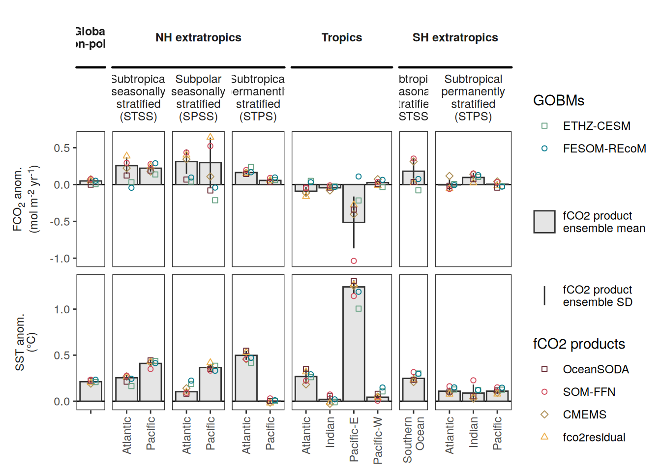
ggsave(width = 10,
       height = 6,
       dpi = 600,
       filename = "../output/biome_anomaly_ensemble_mean_pco2_products.pdf")


p_global <- pco2_product_biome_annual_anomaly_merged_ensemble %>%
  filter(biome == "Global non-polar") %>%
  ggplot(aes(basin, resid)) +
  geom_hline(yintercept = 0) +
  geom_col(aes(fill = "fCO2 product\nensemble mean"), col = "grey20") +
  geom_linerange(aes(ymin = resid - resid_sd,
                     ymax = resid + resid_sd,
                     col = "fCO2 product\nensemble SD")) +
  scale_color_manual(values = "grey20", name = "") +
  scale_fill_manual(values = "grey90", name = "") +
  new_scale_color()+
  geom_point(
    data = pco2_product_biome_annual_anomaly_merged %>%
      filter(biome == "Global non-polar",
             product %in% pco2_product_list),
    aes(col = product),
    # position = position_nudge(x = -0.15),
    shape = 21
  ) +
  scale_color_manual(values = color_products,
                     name = "fCO2 products") +
  new_scale_color()+
  geom_point(data = pco2_product_biome_annual_anomaly_merged %>%
               filter(biome == "Global",
                      product %in% gobm_product_list),
             aes(col = product),
             position = position_nudge(x = 0.2),
             shape = 21) +
  scale_color_manual(values = color_products,
                     name = "GOBMs") +
  facet_nested(name ~ latitude + biome_class,
             scales = "free", space = "free_x",
             labeller = labeller(name = x_axis_labels),
             switch = "y",
             nest_line = element_line(),
             solo_line = TRUE) +
  theme(
    axis.text.x = element_text(
      angle = 90,
      vjust = 0.5,
      hjust = 1
    ),
    axis.title.x = element_blank(),
    axis.title.y = element_blank(),
    strip.text.y.left = element_markdown(),
    strip.placement = "outside",
    strip.background.y = element_blank(),
    strip.background.x = element_blank(),
    legend.position = "none"
  )

p_biome <- pco2_product_biome_annual_anomaly_merged_ensemble %>%
  filter(biome != "Global non-polar") %>%
  ggplot(aes(basin, resid)) +
  geom_hline(yintercept = 0) +
  geom_col(aes(fill = "fCO2 product\nensemble mean"), col = "grey20") +
  geom_linerange(aes(ymin = resid - resid_sd,
                     ymax = resid + resid_sd,
                     col = "fCO2 product\nensemble SD")) +
  scale_color_manual(values = "grey20", name = "") +
  scale_fill_manual(values = "grey90", name = "") +
  new_scale_color()+
  geom_point(
    data = pco2_product_biome_annual_anomaly_merged %>%
      filter(biome != "Global non-polar",
             product %in% pco2_product_list),
    aes(col = product),
    # position = position_nudge(x = -0.15),
    shape = 21
  ) +
  scale_color_manual(values = color_products,
                     name = "fCO2 products") +
  new_scale_color()+
  geom_point(data = pco2_product_biome_annual_anomaly_merged %>%
               filter(biome != "Global non-polar",
                      product %in% gobm_product_list),
             aes(col = product),
             position = position_nudge(x = 0.2),
             shape = 21) +
  scale_color_manual(values = color_products,
                     name = "GOBMs") +
  facet_nested(name ~ latitude + biome_class,
             scales = "free", space = "free_x",
             labeller = labeller(name = ""),
             # switch = "y",
             nest_line = element_line(),
             solo_line = TRUE
             ) +
  theme(
    axis.text.x = element_text(
      angle = 90,
      vjust = 0.5,
      hjust = 1
    ),
    axis.title.x = element_blank(),
    axis.title.y = element_blank(),
    strip.text.y.right = element_text(colour = "transparent",
                                      size = 0),
    strip.placement = "outside",
    strip.background.y = element_blank(),
    strip.background.x = element_blank(),
    legend.position = "bottom",
    legend.direction = "vertical"
  )


ggsave(cowplot::plot_grid(p_global, p_biome,
                   align = "hv",
                   axis = "tb",
                   rel_widths = c(1,7)),
       width = 12,
       height = 8,
       dpi = 600,
       filename = "../output/biome_anomaly_ensemble_mean_pco2_products_with_integrated_flux_and_SO.pdf")
Seasonal anomalies
Annual mean trends
pco2_product_biome_monthly_detrended %>%
  filter(biome %in% "NA-STPS",
         name %in% c("temperature"),
         product %in% pco2_product_list) %>%
  select(-c(time, product)) %>%
  group_by(year, month, biome, name) %>%
  summarise(across(where(is.numeric), mean)) %>%
  ungroup()
# A tibble: 408 × 7
year month biome name value fit resid
<dbl> <dbl> <chr> <fct> <dbl> <dbl> <dbl>
1 1990 1 NA-STPS temperature 23.4 23.4 -0.0569
2 1990 2 NA-STPS temperature 22.9 22.9 0.0174
3 1990 3 NA-STPS temperature 22.8 22.9 -0.0959
4 1990 4 NA-STPS temperature 23.2 23.3 -0.0743
5 1990 5 NA-STPS temperature 24.3 24.2 0.0880
6 1990 6 NA-STPS temperature 25.3 25.4 -0.0876
7 1990 7 NA-STPS temperature 26.3 26.3 -0.0783
8 1990 8 NA-STPS temperature 27.1 27.0 0.0741
9 1990 9 NA-STPS temperature 27.4 27.2 0.155
10 1990 10 NA-STPS temperature 26.9 26.7 0.184
# ℹ 398 more rowspco2_product_biome_monthly_detrended %>%
filter(biome %in% "Global non-polar",
name %in% c("temperature"),
product %in% pco2_product_list) %>%
select(-c(time, product)) %>%
group_by(year, month, biome, name) %>%
summarise(across(where(is.numeric), mean)) %>%
ungroup() %>%
# mutate(product = "Ensemble mean") %>%
p_season(title = NULL,
dim_col = NULL) +
theme(legend.position = "none")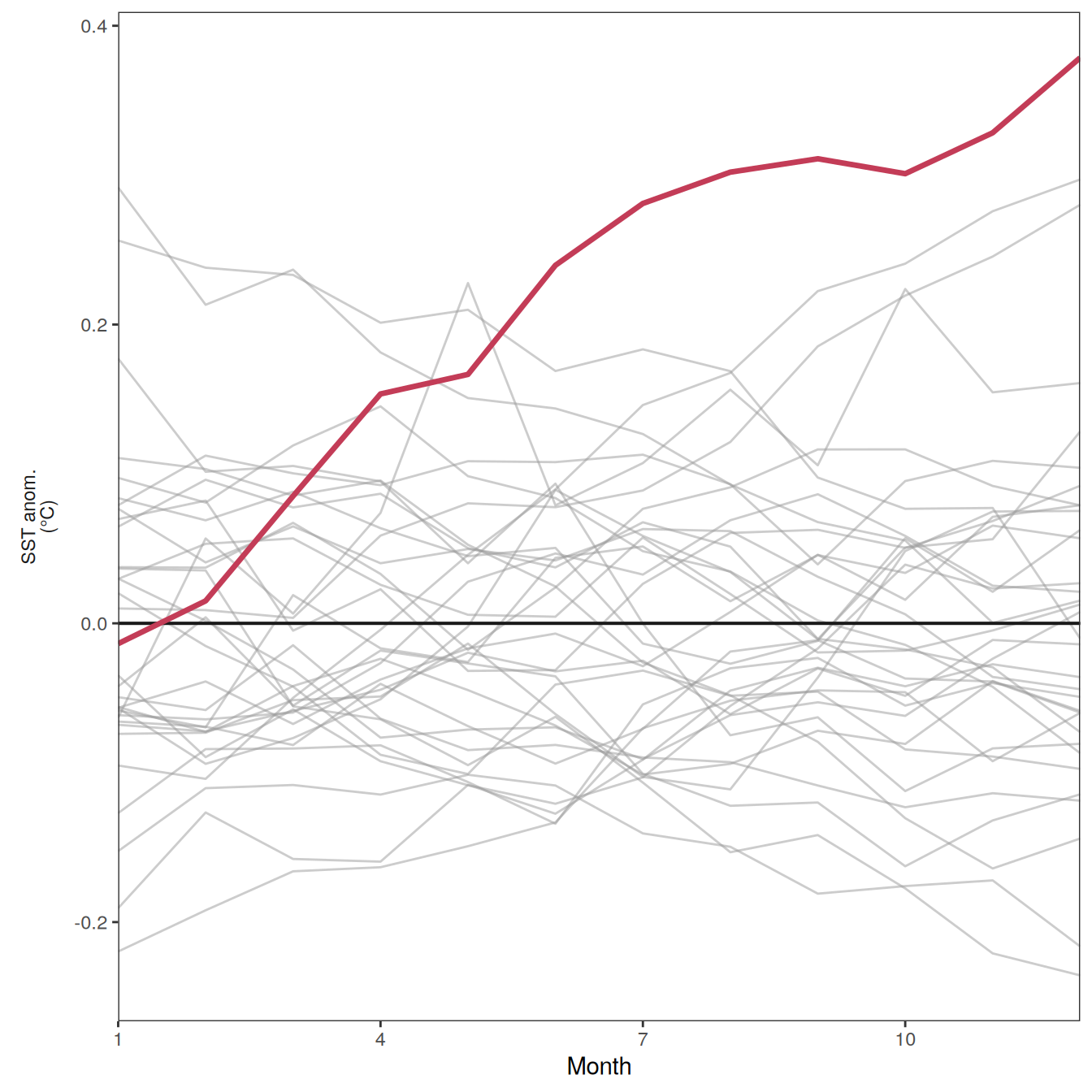
ggsave(width = 5,
       height = 2,
       dpi = 600,
       filename = "../output/global_seasonality_sst_ensemble_mean_pco2_products.pdf")

pco2_product_biome_monthly_detrended %>%
  filter(biome %in% "Global non-polar",
         name %in% c("fgco2_int"),
         product %in% pco2_product_list) %>%
  select(-c(time, product)) %>%
  group_by(year, month, biome, name) %>%
  summarise(across(where(is.numeric), mean)) %>%
  ungroup() %>%
  # mutate(product = "Ensemble mean") %>%
  p_season(title = NULL,
           dim_col = NULL) +
  theme(legend.position = "none")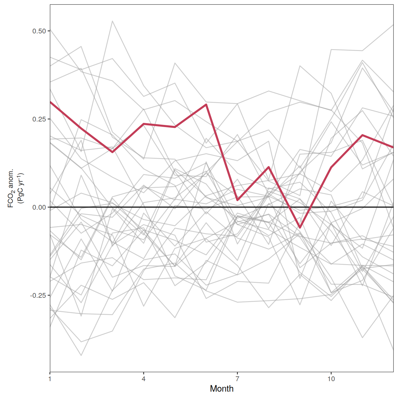
ggsave(width = 5,
       height = 2,
       dpi = 600,
       filename = "../output/global_seasonality_fgco2_ensemble_mean_pco2_products.pdf")
pco2_product_biome_annual_detrended %>%
filter(biome %in% "Global non-polar",
name %in% c("fgco2", "temperature")) %>%
p_season(title = NULL) +
theme(legend.position = "top")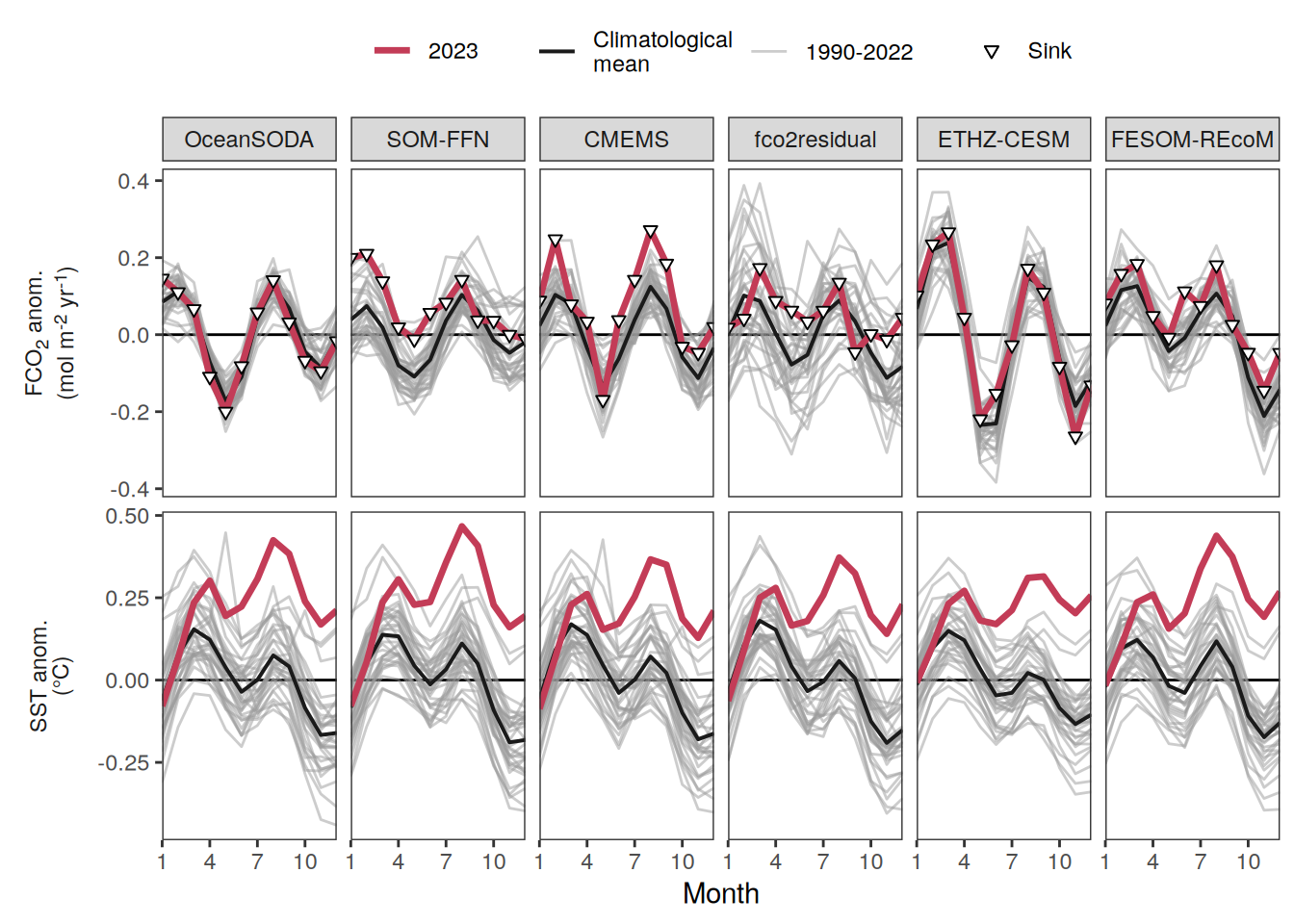
ggsave(width = 10,
       height = 4,
       dpi = 600,
       filename = "../output/global_seasonality_sst_all_products.pdf")
pco2_product_biome_annual_detrended %>%
filter(biome %in% "Global non-polar", name %in% name_core) %>%
p_season(title = "Anomalies from predicted annual mean | Global non-polar")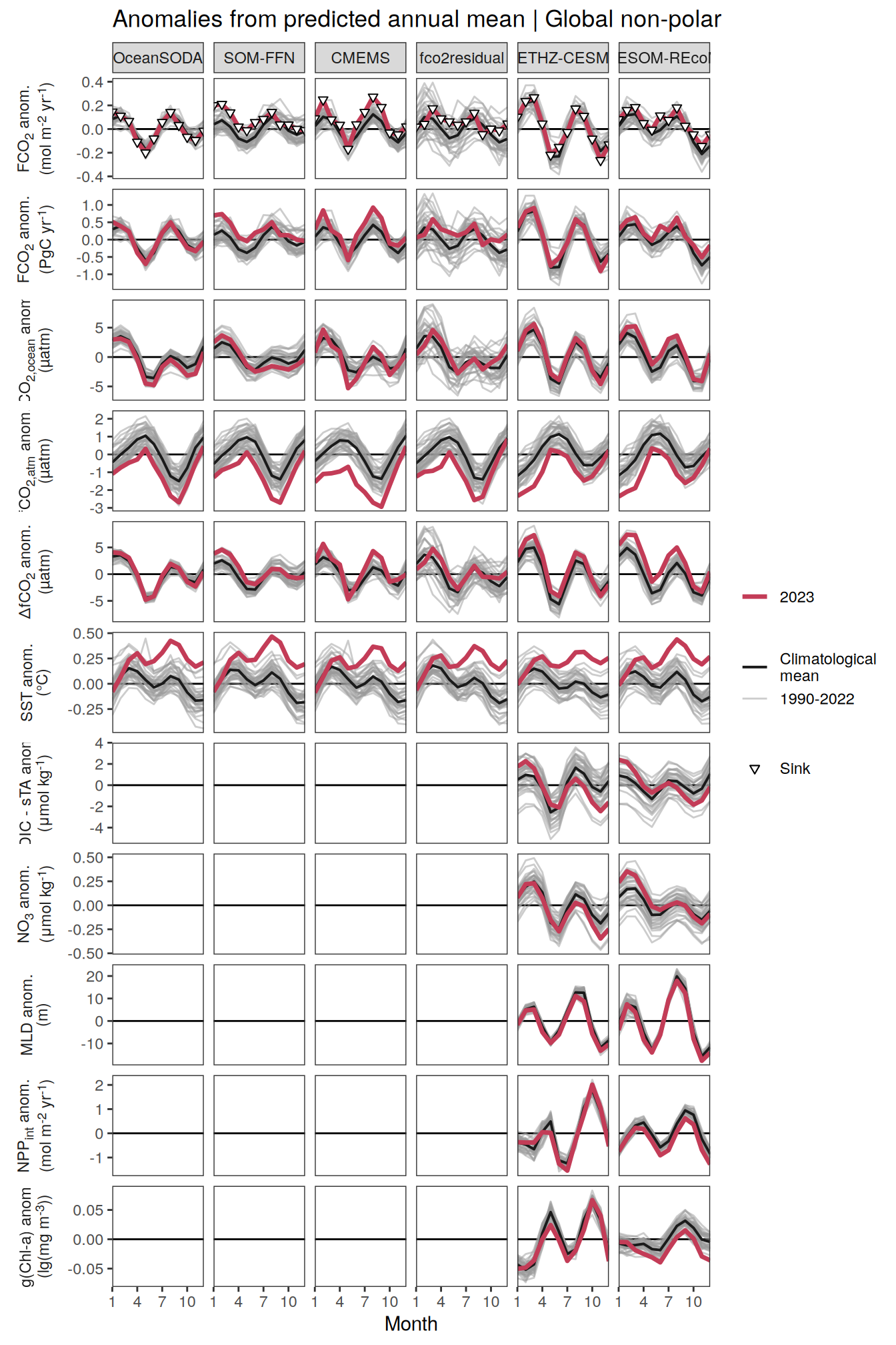
pco2_product_biome_annual_detrended %>%
  filter(biome %in% key_biomes,
         name %in% name_core) %>%
  group_split(biome) %>%
  # head(1) %>%
  map(~ p_season(
    df = .x,
    title = paste("Anomalies from predicted annual mean |", .x$biome)
  ))
[[1]]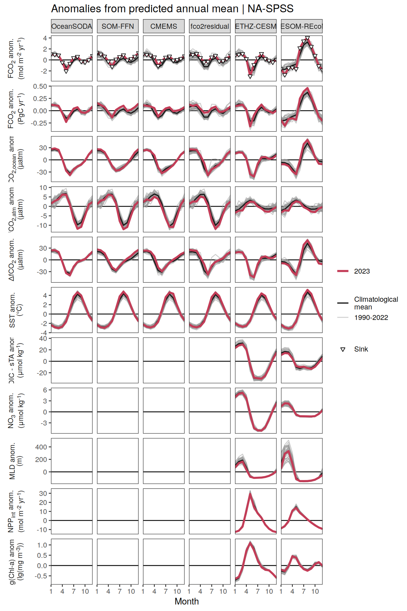
[[2]]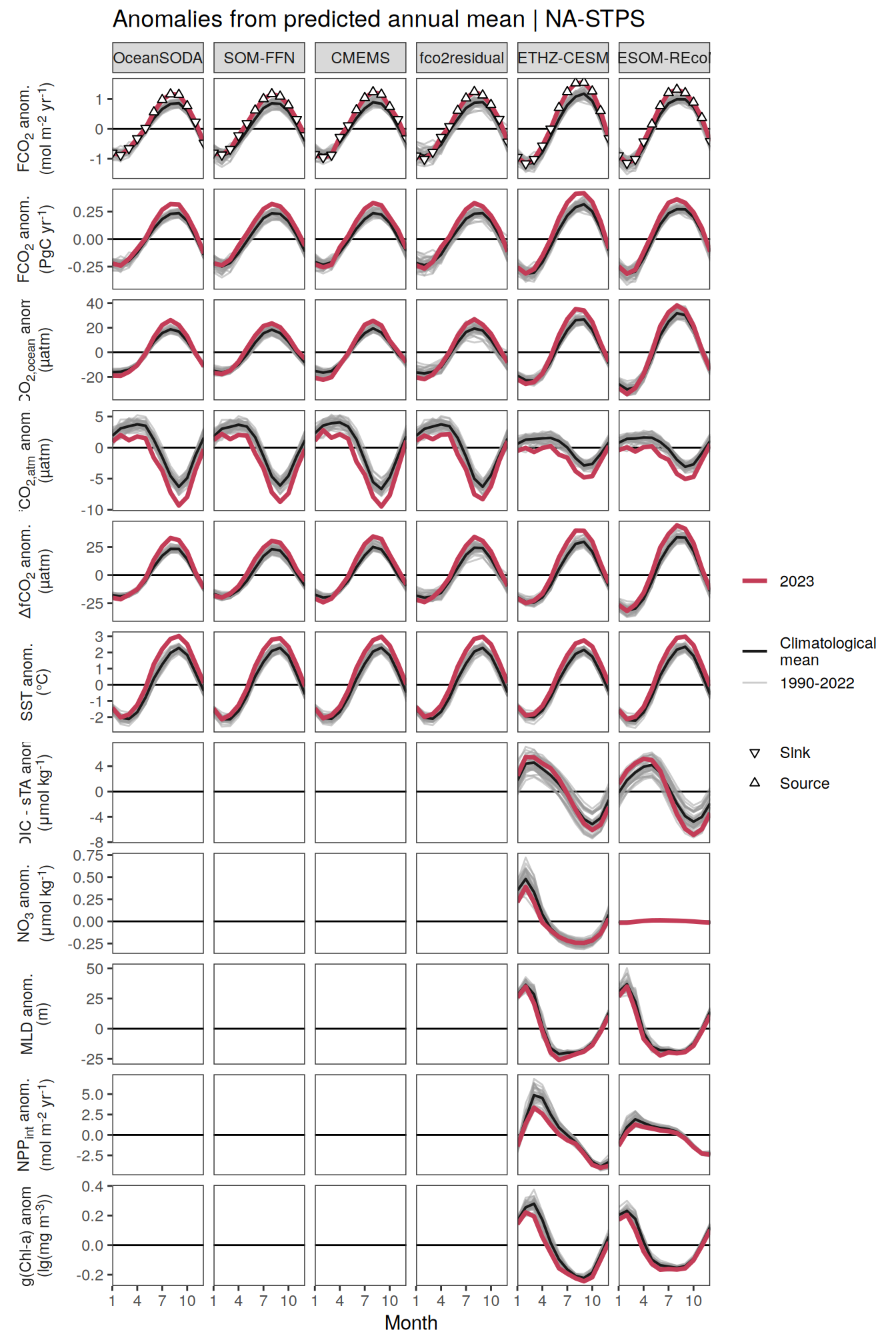
[[3]]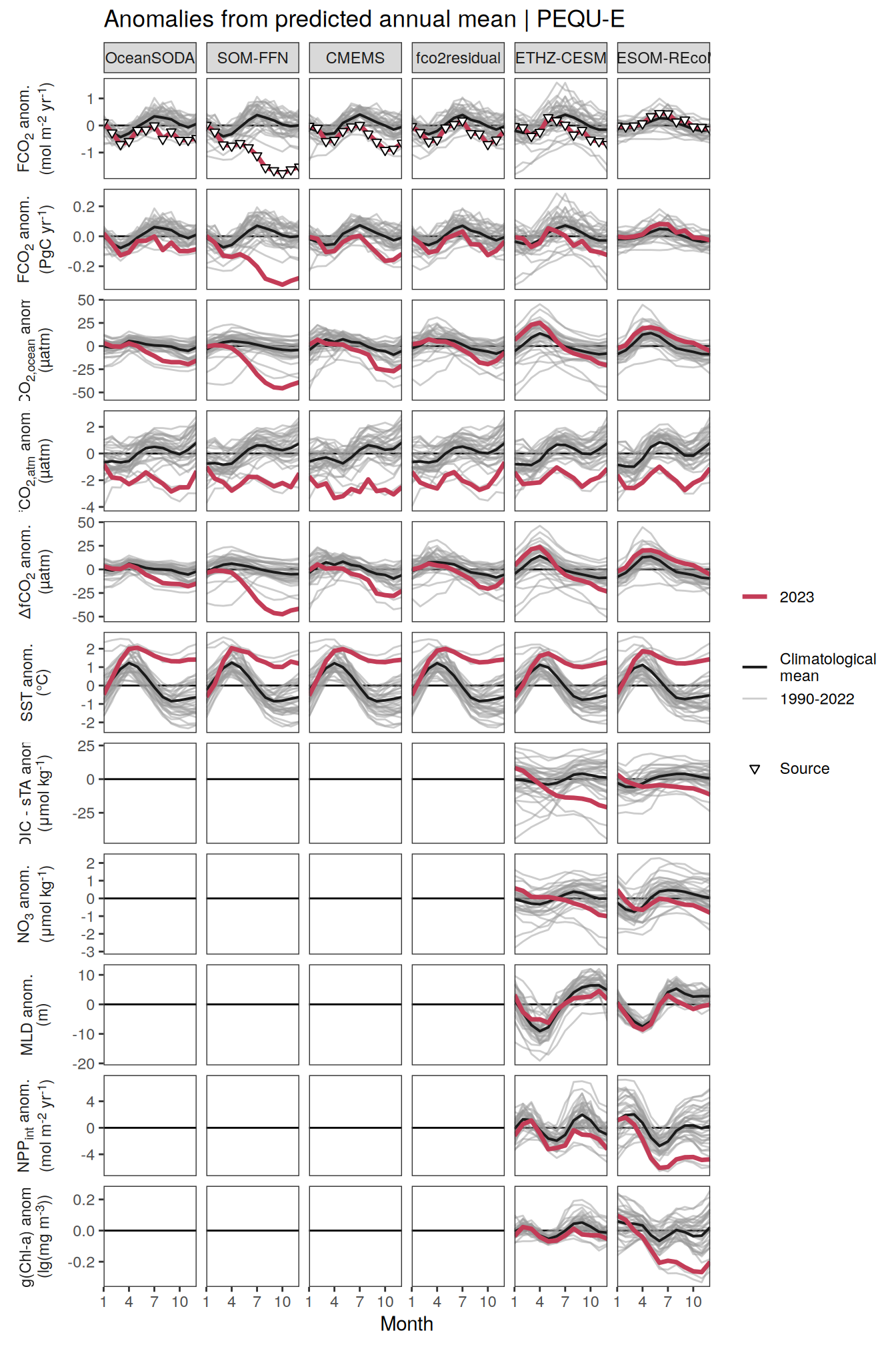
Monthly mean trends
grDevices::cairo_pdf("../output/biome_seasonality_all_products.pdf",
    width = 9,
    height = 10,
    onefile = TRUE)

pco2_product_biome_monthly_detrended %>%
  filter(biome %in% c("Global non-polar", key_biomes),
         name %in% name_core) %>%
  group_split(biome) %>%
  # head(1) %>%
  map(~ p_season(
    df = .x,
    title = paste("Anomalies from predicted monthly mean |", .x$biome)
  ))
[[1]]
[[2]]
[[3]]
[[4]]dev.off()png
2 Flux anomaly correlation
The following plots aim to unravel the correlation between biome-, super-biome- or globally- integrated monthly flux anomalies and the corresponding anomalies of the means/integrals of each other variable.
Anomalies are first presented are first presented in absolute units. Due to the different flux magnitudes, we need to plot the globally and biome-integrated fluxes separately. Secondly, we normalize the anomalies to the monthly spread (expressed as standard deviation) of the anomalies from 1990 to 2021.
Annual anomalies
Absolute
pco2_product_biome_annual_anomaly %>%
  filter(biome %in% c("Global non-polar", key_biomes),
         name %in% name_core) %>%
  mutate(biome = if_else(biome == "Global non-polar", "Global non-polar", biome)) %>%
  select(-c(value, fit)) %>%
  pivot_wider(values_from = resid) %>%
  pivot_longer(-c(product, year, biome, fgco2_int))  %>%
  filter(name == "temperature") %>%
  group_split(name) %>%
  # tail(1) %>%
  map(
    ~ ggplot(data = .x,
             aes(value, fgco2_int)) +
      geom_smooth(
        data = . %>% filter(year != 2023),
        method = "lm",
        fill = "grey",
        col = "grey40",
        fullrange = TRUE,
        level = 0.68
      ) +
      geom_point(
        data = . %>% filter(!year %in% c(2023, 1997, 2015)),
        aes(fill = "1990-2022"),
        shape = 21
      ) +
      scale_color_manual(values = "grey60", name = "X") +
      scale_fill_manual(values = "grey60", name = "X") +
      new_scale_fill() +
      new_scale_color() +
      geom_point(
        data = . %>% filter(year %in% c(2023, 1997, 2015)),
        aes(fill = as.factor(year)),
        shape = 21,
        size = 3
      )  +
      scale_fill_manual(
        values = rev(warm_cool_gradient[c(17,13,20)]),
        guide = guide_legend(reverse = TRUE,
                             order = 2)
      ) +
      scale_color_manual(
        values = rev(warm_cool_gradient[c(17,13,20)]),
        guide = guide_legend(reverse = TRUE,
                             order = 2)
      ) +
      labs(y = labels_breaks("fgco2_int")$i_legend_title,
           x = labels_breaks(unique(.x$name))$i_legend_title) +
      facet_grid2(
        product ~ biome,
        scales = "free",
        independent = "y"
      ) +
      theme(
        axis.title.x = element_markdown(),
        axis.title.y = element_markdown(),
        legend.title = element_blank(),
        legend.position = "top"
      )
  )
[[1]]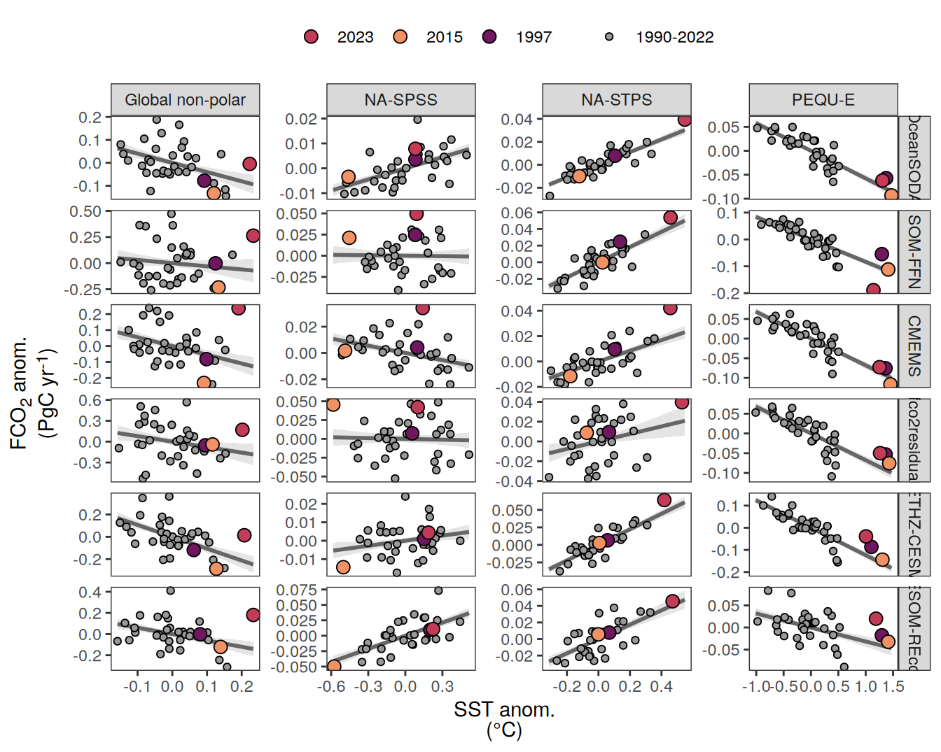
ggsave(width = 8,
       height = 10,
       dpi = 600,
       filename = "../output/biome_anomaly_correlation_all_pco2_products.pdf")


pco2_product_biome_annual_anomaly_ensemble <-
  pco2_product_biome_annual_anomaly %>%
  filter(name %in% name_core, product %in% pco2_product_list) %>%
  select(-c(value, fit, product)) %>%
  fgroup_by(name, biome, year) %>%
  fsummarise(sd = fsd(resid),
             mean = fmean(resid))

pco2_product_biome_annual_anomaly_ensemble <-
  full_join(
    pco2_product_biome_annual_anomaly_ensemble %>%
      filter(name == "fgco2_int") %>%
      pivot_wider(values_from = c(sd, mean)),
    pco2_product_biome_annual_anomaly_ensemble %>%
      filter(name != "fgco2_int")
  )


pco2_product_biome_annual_anomaly_super_regions %>%
  filter(name %in% c("fgco2_int", "temperature")) %>%
  select(-contains("value")) %>%
  pivot_wider(values_from = contains("resid")) %>%
  filter(biome %in% c("Global non-polar", key_biomes)) %>%
  ggplot(aes(resid_temperature, resid_fgco2_int)) +
  # geom_vline(xintercept = 0) +
  # geom_hline(yintercept = 0) +
  geom_smooth(
    data = . %>% filter(year != 2023),
    method = "lm",
    fill = "grey",
    col = "grey40",
    fullrange = TRUE,
    level = 0.68
  )+
  geom_linerange(
    data = . %>% filter(!year %in% c(2023, 1997, 2015)),
    aes(
      ymin = resid_fgco2_int - resid_sd_fgco2_int,
      ymax = resid_fgco2_int + resid_sd_fgco2_int,
      col = "1990-2022"
    )
  ) +
  geom_linerange(
    data = . %>% filter(!year %in% c(2023, 1997, 2015)),
    aes(
      xmin = resid_temperature - resid_sd_temperature,
      xmax = resid_temperature + resid_sd_temperature,
      col = "1990-2022"
    )
  ) +
  geom_point(data = . %>% filter(!year %in% c(2023, 1997, 2015)),
             aes(fill = "1990-2022"),
             shape = 21) +
  scale_color_manual(values = "grey60", name = "X") +
  scale_fill_manual(values = "grey60", name = "X") +
  new_scale_fill() +
  new_scale_color() +
  geom_linerange(
    data = . %>% filter(year %in% c(2023, 1997, 2015)),
    aes(
      ymin = resid_fgco2_int - resid_sd_fgco2_int,
      ymax = resid_fgco2_int + resid_sd_fgco2_int,
      col = as.factor(year)
    ),
    linewidth = 1
  ) +
  geom_linerange(
    data = . %>% filter(year %in% c(2023, 1997, 2015)),
    aes(
      xmin = resid_temperature - resid_sd_temperature,
      xmax = resid_temperature + resid_sd_temperature,
      col = as.factor(year)
    ),
    linewidth = 1
  ) +
  geom_point(
    data = . %>% filter(year %in% c(2023, 1997, 2015)),
    aes(fill = as.factor(year)),
    shape = 21,
    size = 3
  )  +
  scale_fill_manual(values = rev(warm_cool_gradient[c(17, 13, 20)]),
                    guide = guide_legend(reverse = TRUE, order = 2)) +
  scale_color_manual(values = rev(warm_cool_gradient[c(17, 13, 20)]),
                     guide = guide_legend(reverse = TRUE, order = 2)) +
  labs(y = labels_breaks("fgco2_int")$i_legend_title,
       x = labels_breaks(unique("temperature"))$i_legend_title) +
  facet_wrap(~ biome, scales = "free") +
  # theme_classic() +
  theme(
    axis.title.x = element_markdown(),
    axis.title.y = element_markdown(),
    legend.title = element_blank()
    # strip.background = element_blank()
  )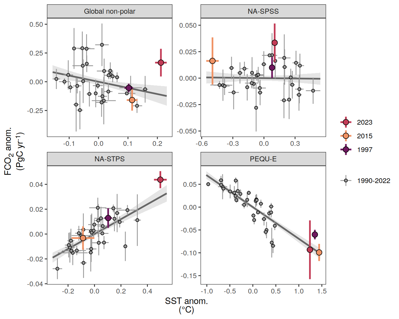
ggsave(width = 8,
       height = 6,
       dpi = 600,
       filename = "../output/Fig2.pdf")

pco2_product_biome_annual_anomaly_super_regions %>%
  filter(name %in% c("fgco2_int", "temperature")) %>%
  select(-contains("value")) %>%
  pivot_wider(values_from = contains("resid")) %>%
  filter(biome %in% c("Global non-polar")) %>%
  ggplot(aes(resid_temperature, resid_fgco2_int)) +
  # geom_vline(xintercept = 0) +
  # geom_hline(yintercept = 0) +
  geom_smooth(
    data = . %>% filter(year != 2023),
    method = "lm",
    fill = "grey",
    col = "grey40",
    fullrange = TRUE,
    level = 0.68
  )+
  geom_linerange(
    data = . %>% filter(!year %in% c(2023, 1997, 2015)),
    aes(
      ymin = resid_fgco2_int - resid_sd_fgco2_int,
      ymax = resid_fgco2_int + resid_sd_fgco2_int,
      col = "1990-2022"
    )
  ) +
  geom_linerange(
    data = . %>% filter(!year %in% c(2023, 1997, 2015)),
    aes(
      xmin = resid_temperature - resid_sd_temperature,
      xmax = resid_temperature + resid_sd_temperature,
      col = "1990-2022"
    )
  ) +
  geom_point(data = . %>% filter(!year %in% c(2023, 1997, 2015)),
             aes(fill = "1990-2022"),
             shape = 21) +
  scale_color_manual(values = "grey60", name = "X") +
  scale_fill_manual(values = "grey60", name = "X") +
  new_scale_fill() +
  new_scale_color() +
  geom_linerange(
    data = . %>% filter(year %in% c(2023, 1997, 2015)),
    aes(
      ymin = resid_fgco2_int - resid_sd_fgco2_int,
      ymax = resid_fgco2_int + resid_sd_fgco2_int,
      col = as.factor(year)
    ),
    linewidth = 1
  ) +
  geom_linerange(
    data = . %>% filter(year %in% c(2023, 1997, 2015)),
    aes(
      xmin = resid_temperature - resid_sd_temperature,
      xmax = resid_temperature + resid_sd_temperature,
      col = as.factor(year)
    ),
    linewidth = 1
  ) +
  geom_point(
    data = . %>% filter(year %in% c(2023, 1997, 2015)),
    aes(fill = as.factor(year)),
    shape = 21,
    size = 3
  )  +
  scale_fill_manual(values = rev(warm_cool_gradient[c(17, 13, 20)]),
                    guide = guide_legend(reverse = TRUE, order = 2)) +
  scale_color_manual(values = rev(warm_cool_gradient[c(17, 13, 20)]),
                     guide = guide_legend(reverse = TRUE, order = 2)) +
  labs(y = labels_breaks("fgco2_int")$i_legend_title,
       x = labels_breaks(unique("temperature"))$i_legend_title) +
  theme(
    axis.title.x = element_markdown(),
    axis.title.y = element_markdown(),
    legend.title = element_blank()
    # strip.background = element_blank()
  )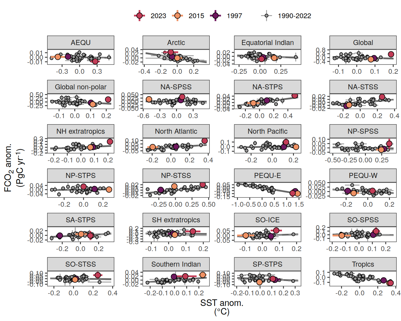
ggsave(width = 5,
       height = 3.5,
       dpi = 900,
       filename = "../output/biome_anomaly_correlation_ensemble_mean_pco2_products_global.pdf")


pco2_product_biome_annual_anomaly_super_regions %>%
  filter(name %in% c("fgco2_int", "temperature")) %>%
  select(-contains("value")) %>%
  pivot_wider(values_from = contains("resid")) %>%
  ggplot(aes(resid_temperature, resid_fgco2_int)) +
  # geom_vline(xintercept = 0) +
  # geom_hline(yintercept = 0) +
  geom_smooth(
    data = . %>% filter(year != 2023),
    method = "lm",
    fill = "grey",
    col = "grey40",
    fullrange = TRUE,
        level = 0.68
  ) +
  geom_linerange(
    data = . %>% filter(!year %in% c(2023, 1997, 2015)),
    aes(
      ymin = resid_fgco2_int - resid_sd_fgco2_int,
      ymax = resid_fgco2_int + resid_sd_fgco2_int,
      col = "1990-2022"
    )
  ) +
  geom_linerange(
    data = . %>% filter(!year %in% c(2023, 1997, 2015)),
    aes(
      xmin = resid_temperature - resid_sd_temperature,
      xmax = resid_temperature + resid_sd_temperature,
      col = "1990-2022"
    )
  ) +
  geom_point(data = . %>% filter(!year %in% c(2023, 1997, 2015)),
             aes(fill = "1990-2022"),
             shape = 21) +
  scale_color_manual(values = "grey60", name = "X") +
  scale_fill_manual(values = "grey60", name = "X") +
  new_scale_fill() +
  new_scale_color() +
  geom_linerange(
    data = . %>% filter(year %in% c(2023, 1997, 2015)),
    aes(
      ymin = resid_fgco2_int - resid_sd_fgco2_int,
      ymax = resid_fgco2_int + resid_sd_fgco2_int,
      col = as.factor(year)
    ),
    linewidth = 1
  ) +
  geom_linerange(
    data = . %>% filter(year %in% c(2023, 1997, 2015)),
    aes(
      xmin = resid_temperature - resid_sd_temperature,
      xmax = resid_temperature + resid_sd_temperature,
      col = as.factor(year)
    ),
    linewidth = 1
  ) +
  geom_point(
    data = . %>% filter(year %in% c(2023, 1997, 2015)),
    aes(fill = as.factor(year)),
    shape = 21,
    size = 3
  )  +
  scale_fill_manual(values = rev(warm_cool_gradient[c(17, 13, 20)]),
                    guide = guide_legend(reverse = TRUE, order = 2)) +
  scale_color_manual(values = rev(warm_cool_gradient[c(17, 13, 20)]),
                     guide = guide_legend(reverse = TRUE, order = 2)) +
  labs(y = labels_breaks("fgco2_int")$i_legend_title,
       x = labels_breaks(unique("temperature"))$i_legend_title) +
  facet_wrap(~ biome, scales = "free",
             ncol = 4) +
  # theme_classic() +
  theme(
    axis.title.x = element_markdown(),
    axis.title.y = element_markdown(),
    legend.title = element_blank(),
    legend.position = "top"
  )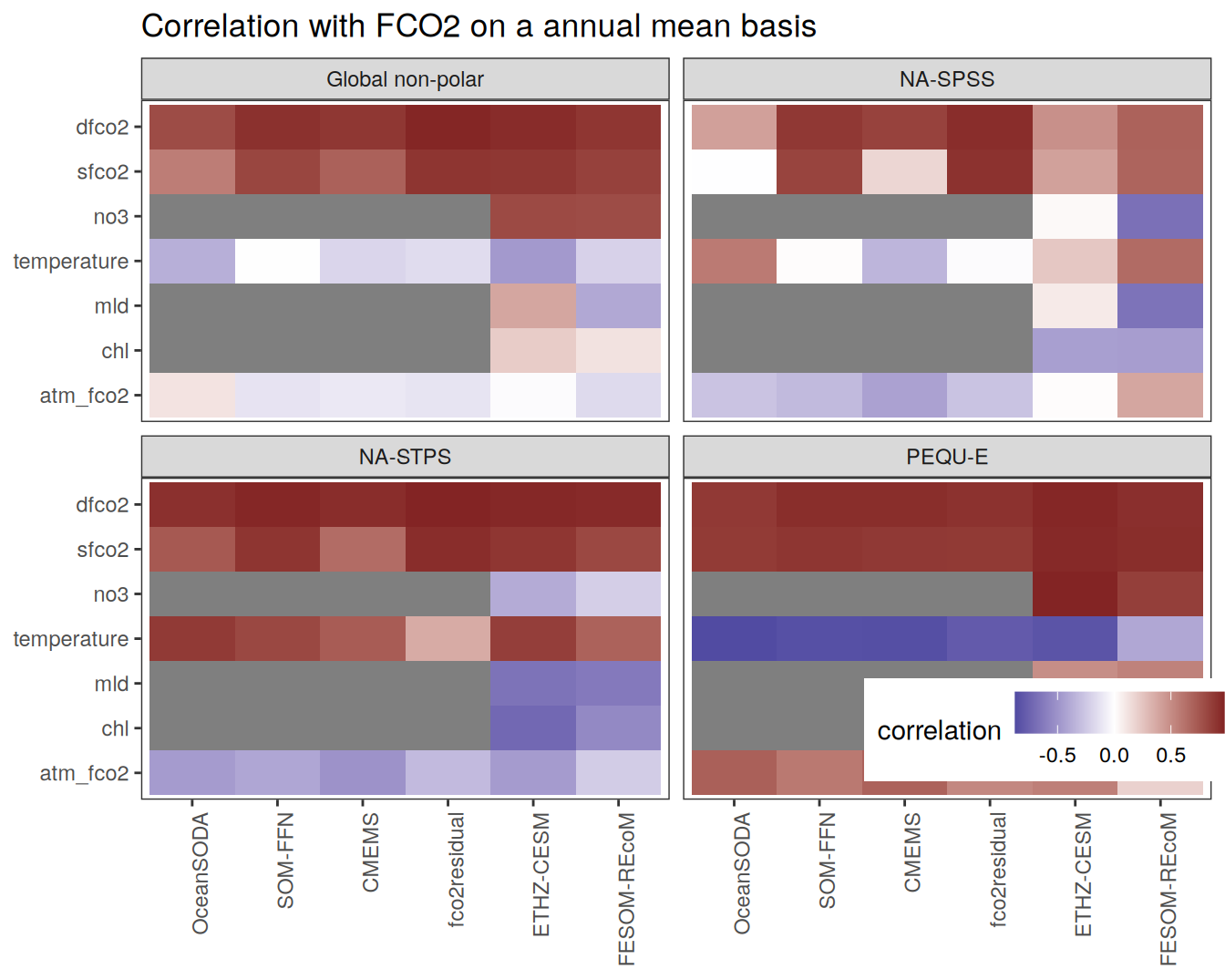
ggsave(width = 9,
       height = 12,
       dpi = 600,
       filename = "../output/biome_anomaly_correlation_ensemble_mean_pco2_products_all_biomes.pdf")


pco2_product_biome_annual_anomaly %>%
  filter(
    biome %in% c("Global non-polar", key_biomes),
    name %in% c(
      "fgco2_int",
      "chl",
      "dfco2",
      "sfco2",
      "atm_fco2",
      "temperature",
      "sdissic",
      "no3",
      "int_pp",
      "mld",
      "kw_sol"
    )
  ) %>%
  select(-c(value, fit)) %>%
  pivot_wider(values_from = resid) %>%
  pivot_longer(-c(product, year, biome, fgco2_int)) %>%
  group_by(product, name, biome) %>%
  summarise(correlation = cor(fgco2_int, value)) %>%
  ungroup() %>%
  group_by(name) %>%
  mutate(correlation_mean = mean(abs(correlation), na.rm = TRUE)) %>%
  ungroup() %>%
  mutate(name = fct_reorder(name, correlation_mean)) %>%
  ggplot(aes(product,name,fill=correlation)) +
  geom_tile() +
  scale_fill_divergent() +
  facet_wrap(~ biome) +
  labs(title = "Correlation with FCO2 on a annual mean basis") +
  theme(axis.text.x = element_text(angle = 90, hjust = 1),
        axis.title = element_blank(),
        legend.position = c(0.85,0.1),
        legend.direction = "horizontal")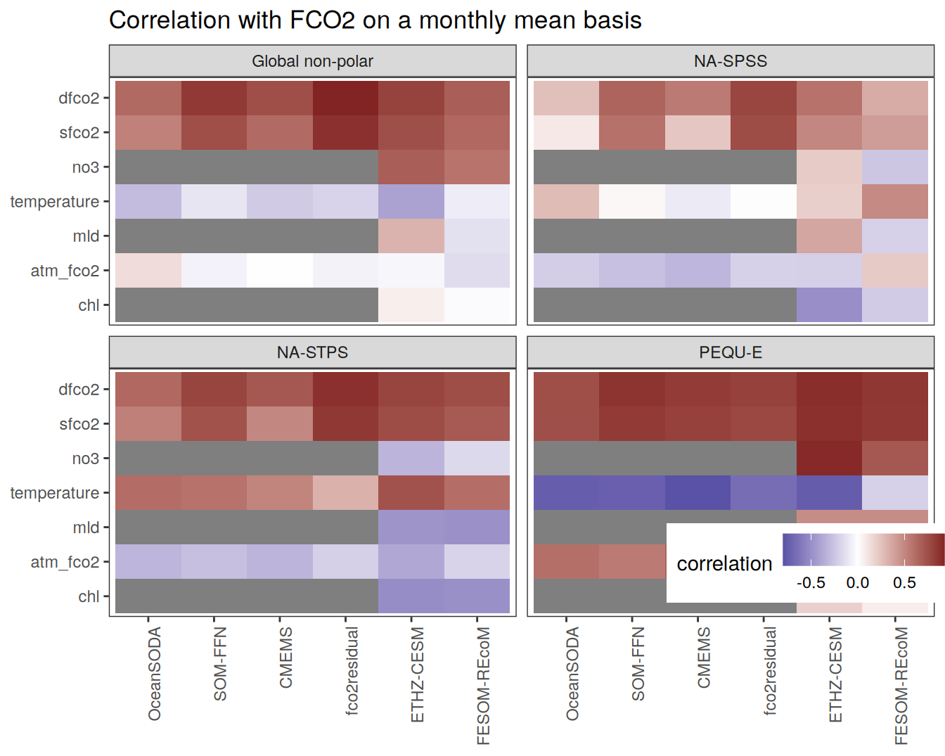
pco2_product_biome_monthly_anomaly %>%
filter(
    biome %in% c("Global non-polar", key_biomes),
    name %in% c(
      "fgco2_int",
      "chl",
      "dfco2",
      "sfco2",
      "atm_fco2",
      "temperature",
      "sdissic",
      "no3",
      "int_pp",
      "mld",
      "kw_sol"
    )
  ) %>%
  select(-c(value, fit)) %>%
  pivot_wider(values_from = resid) %>%
  pivot_longer(-c(product, year, month, biome, fgco2_int)) %>%
  group_by(product, name, biome) %>%
  summarise(correlation = cor(fgco2_int, value)) %>%
  ungroup() %>%
  group_by(name) %>%
  mutate(correlation_mean = mean(abs(correlation), na.rm = TRUE)) %>%
  ungroup() %>%
  mutate(name = fct_reorder(name, correlation_mean)) %>%
  ggplot(aes(product,name,fill=correlation)) +
  geom_tile() +
  scale_fill_divergent() +
  facet_wrap(~ biome) +
  labs(title = "Correlation with FCO2 on a monthly mean basis") +
  theme(axis.text.x = element_text(angle = 90, hjust = 1),
        axis.title = element_blank(),
        legend.position = c(0.85,0.1),
        legend.direction = "horizontal")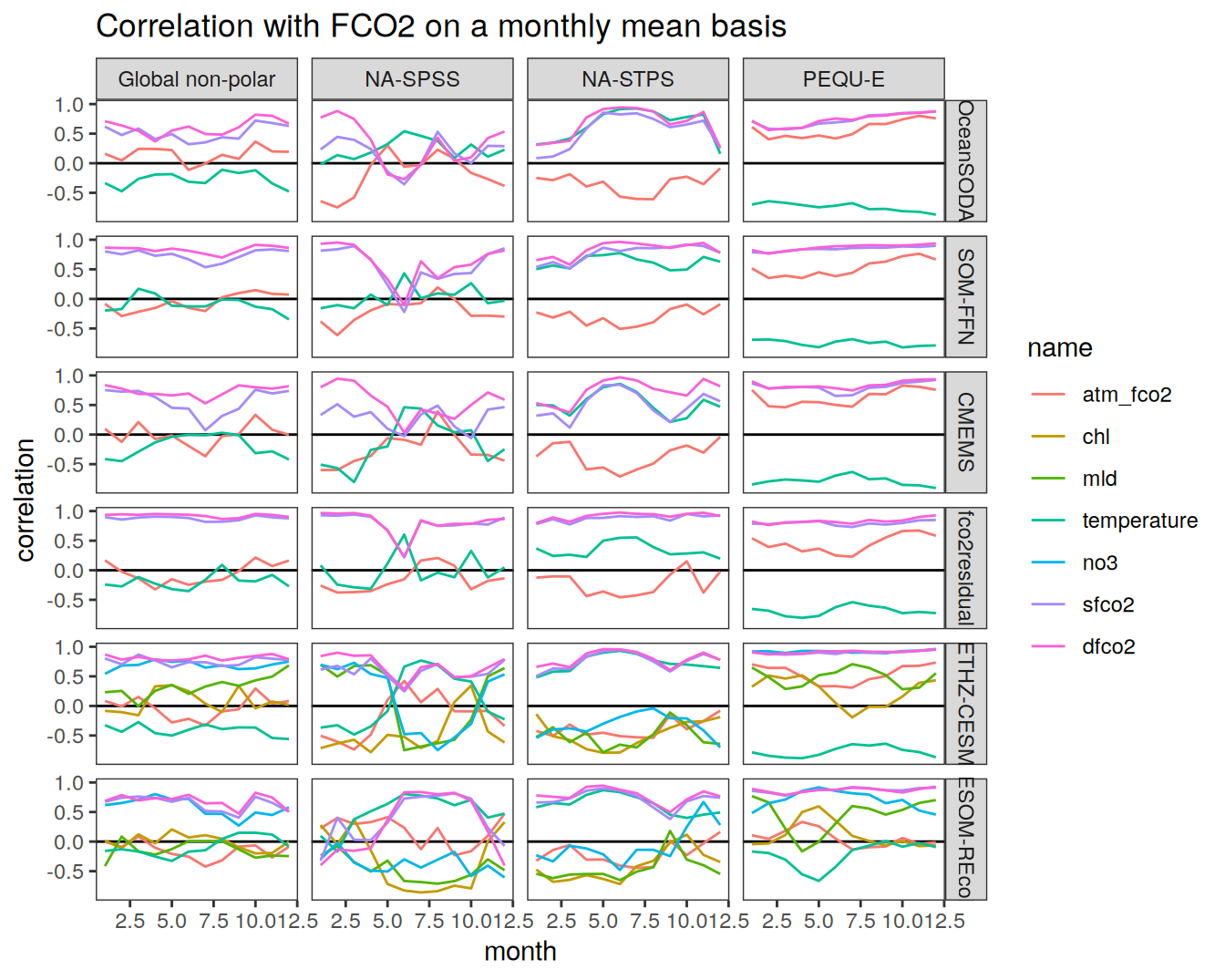
pco2_product_biome_monthly_anomaly %>%
filter(
    biome %in% c("Global non-polar", key_biomes),
    name %in% c(
      "fgco2_int",
      "chl",
      "dfco2",
      "sfco2",
      "atm_fco2",
      "temperature",
      "sdissic",
      "no3",
      "int_pp",
      "mld",
      "kw_sol"
    )
  ) %>%
  select(-c(value, fit)) %>%
  pivot_wider(values_from = resid) %>%
  pivot_longer(-c(product, year, month, biome, fgco2_int)) %>%
  group_by(product, name, biome, month) %>%
  summarise(correlation = cor(fgco2_int, value)) %>%
  ungroup() %>%
  group_by(name) %>%
  mutate(correlation_mean = mean(abs(correlation), na.rm = TRUE)) %>%
  ungroup() %>%
  mutate(name = fct_reorder(name, correlation_mean)) %>%
  ggplot(aes(month, correlation, col = name)) +
  geom_hline(yintercept = 0) +
  geom_path() +
  facet_grid(product ~ biome) +
  labs(title = "Correlation with FCO2 on a monthly mean basis")
| Version | Author | Date |
|---|---|---|
| 265b0a8 | jens-daniel-mueller | 2025-06-06 |
SST based prediction
pco2_product_biome_annual_anomaly_temperature_predict <-
  full_join(
    pco2_product_biome_annual_anomaly_temperature_predict,
    pco2_product_biome_annual_anomaly_temperature_predict %>%
      filter(year != 2023) %>%
      nest(data = -c(product, biome)) %>%
      mutate(fit = map(
        data, ~ flm(formula = fgco2_int ~ temperature, data = .x)
      )) %>%
      unnest_wider(fit) %>%
      select(product, biome, slope = temperature) %>%
      mutate(slope = as.vector(slope))
  )

pco2_product_biome_annual_anomaly_temperature_predict <-
  pco2_product_biome_annual_anomaly_temperature_predict %>%
  mutate(fgco2_predict_int_biome = slope * temperature)

pco2_product_biome_annual_anomaly_temperature_predict %>%
  select(product,
         year,
         biome,
         `true anomaly` = fgco2_int,
         `SST pattern` = fgco2_predict_int,
         `SST mean` = fgco2_predict_int_biome) %>%
  pivot_longer(4:6,
               values_to = "resid") %>%
  filter(biome %in% c("Global non-polar")) %>%
  ggplot(aes(year, resid))+
  geom_hline(yintercept = 0) +
  geom_path(aes(col = name))+
  geom_point(aes(fill = name), shape = 21, size = 1) +
  labs(y = labels_breaks("fgco2_int")$i_legend_title) +
  facet_wrap( ~ product) +
  theme(
    axis.title.x = element_blank(),
    axis.title.y = element_markdown(),
    legend.title = element_blank()
  )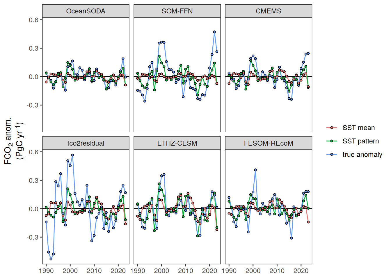
ggsave(width = 10,
       height = 6,
       dpi = 600,
       filename = "../output/biome_flux_anomaly_prediction_timeseries_all_pco2_products_global.pdf")


pco2_product_biome_annual_anomaly_temperature_predict %>%
  filter(year == 2023,
         biome == "Global non-polar",
         product %in% pco2_product_list) %>%
  select(product,
         year,
         biome,
         `true anomaly` = fgco2_int,
         `SST pattern` = fgco2_predict_int,
         `SST mean` = fgco2_predict_int_biome) %>%
  pivot_longer(4:6,
               values_to = "resid") %>%
  group_by(name) %>%
  summarise(sd = sd(resid),
            mean = mean(resid)) %>%
  ungroup()
# A tibble: 3 × 3
name sd mean
<chr> <dbl> <dbl>
1 SST mean 0.0383 -0.106
2 SST pattern 0.0198 -0.0986
3 true anomaly 0.122 0.168 pco2_product_biome_annual_anomaly_temperature_predict %>%
select(product,
year,
biome,
fgco2_int,
`SST pattern` = fgco2_predict_int,
`SST mean` = fgco2_predict_int_biome) %>%
pivot_longer(contains("SST"),
values_to = "resid") %>%
filter(biome %in% c("Global non-polar")) %>%
ggplot(aes(fgco2_int, resid))+
geom_vline(xintercept = 0) +
geom_hline(yintercept = 0) +
geom_smooth(
data = . %>% filter(year != 2023),
method = "lm",
fill = "grey",
col = "grey40",
fullrange = TRUE,
level = 0.68
) +
geom_point(data = . %>% filter(!year %in% c(2023, 1997, 2015)),
aes(fill = "1990-2022"),
shape = 21) +
scale_color_manual(values = "grey60", name = "X") +
scale_fill_manual(values = "grey60", name = "X") +
new_scale_fill() +
new_scale_color() +
geom_point(
data = . %>% filter(year %in% c(2023, 1997, 2015)),
aes(fill = as.factor(year)),
shape = 21,
size = 3
) +
scale_fill_manual(values = rev(warm_cool_gradient[c(17, 13, 20)]),
guide = guide_legend(reverse = TRUE, order = 2)) +
scale_color_manual(values = rev(warm_cool_gradient[c(17, 13, 20)]),
guide = guide_legend(reverse = TRUE, order = 2)) +
labs(x = labels_breaks("fgco2_int")$i_legend_title,
y = labels_breaks("fgco2_predict_int")$i_legend_title) +
facet_grid(name ~ product) +
coord_equal() +
theme(
axis.title.x = element_markdown(),
axis.title.y = element_markdown(),
legend.title = element_blank(),
legend.position = "top"
)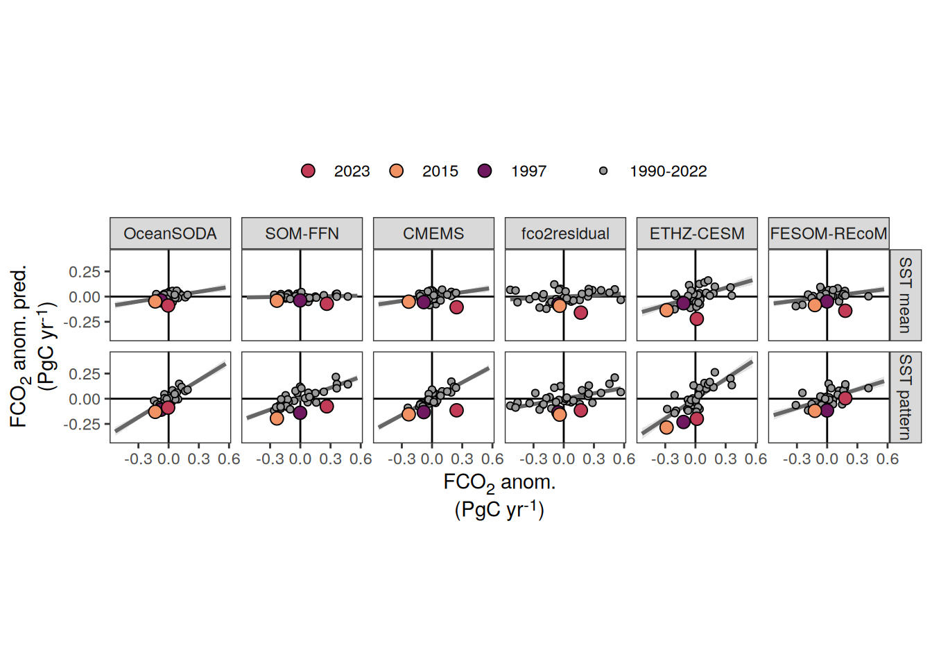
ggsave(width = 10,
       height = 4,
       dpi = 600,
       filename = "../output/biome_flux_anomaly_prediction_correlation_all_pco2_products_global.pdf")


pco2_product_biome_annual_anomaly_temperature_predict %>%
  select(product,
         year,
         biome,
         fgco2_int,
         `SST pattern` = fgco2_predict_int,
         `SST mean` = fgco2_predict_int_biome) %>%
  pivot_longer(contains("SST"),
               values_to = "resid") %>%
  filter(biome %in% c("Global non-polar")) %>%
  group_by(product, biome, name) %>%
  summarise(correlation = cor(fgco2_int, resid)) %>%
  ungroup() %>%
  ggplot(aes(name, correlation, fill = name))+
  geom_hline(yintercept = 0) +
  geom_col(col = "grey20") +
  scale_fill_highcontrast() +
  labs(y = "FCO<sub>2</sub> anom.<br>correlation") +
  facet_grid( ~ product) +
  theme(
    axis.title.x = element_blank(),
    axis.text.x = element_blank(),
    axis.title.y = element_markdown(),
    legend.title = element_blank()
  )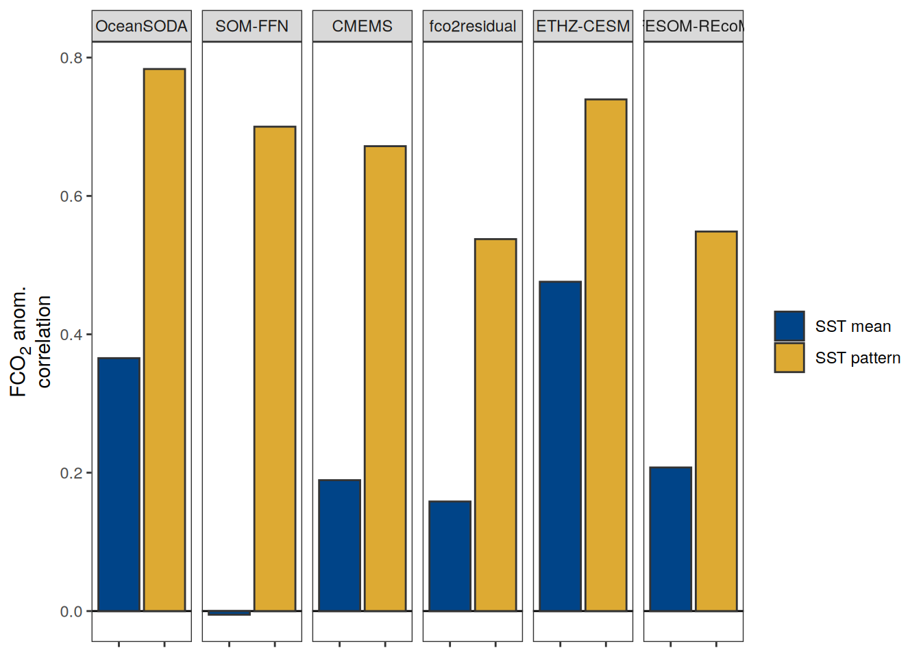
ggsave(width = 10,
       height = 2,
       dpi = 600,
       filename = "../output/biome_flux_anomaly_prediction_correlation_coefficients_all_pco2_products_global.pdf")

pco2_product_biome_annual_anomaly_temperature_predict %>%
  select(product,
         year,
         biome,
         fgco2_int,
         `SST pattern` = fgco2_predict_int) %>%
  pivot_longer(contains("SST"),
               values_to = "resid") %>%
  filter(biome %in% c(key_biomes)) %>%
  ggplot(aes(fgco2_int, resid))+
  geom_vline(xintercept = 0) +
  geom_hline(yintercept = 0) +
  geom_smooth(
    data = . %>% filter(year != 2023),
    method = "lm",
    fill = "grey",
    col = "grey40",
    fullrange = TRUE,
    level = 0.68
  ) +
  geom_point(data = . %>% filter(!year %in% c(2023, 1997, 2015)),
             aes(fill = "1990-2022"),
             shape = 21) +
  scale_color_manual(values = "grey60", name = "X") +
  scale_fill_manual(values = "grey60", name = "X") +
  new_scale_fill() +
  new_scale_color() +
  geom_point(
    data = . %>% filter(year %in% c(2023, 1997, 2015)),
    aes(fill = as.factor(year)),
    shape = 21,
    size = 3
  )  +
  scale_fill_manual(values = rev(warm_cool_gradient[c(17, 13, 20)]),
                    guide = guide_legend(reverse = TRUE, order = 2)) +
  scale_color_manual(values = rev(warm_cool_gradient[c(17, 13, 20)]),
                     guide = guide_legend(reverse = TRUE, order = 2)) +
  labs(x = labels_breaks("fgco2_int")$i_legend_title,
       y = labels_breaks("fgco2_predict_int")$i_legend_title) +
  facet_grid(biome ~ product) +
  coord_equal() +
  theme(
    axis.title.x = element_markdown(),
    axis.title.y = element_markdown(),
    legend.title = element_blank(),
    legend.position = "top"
  )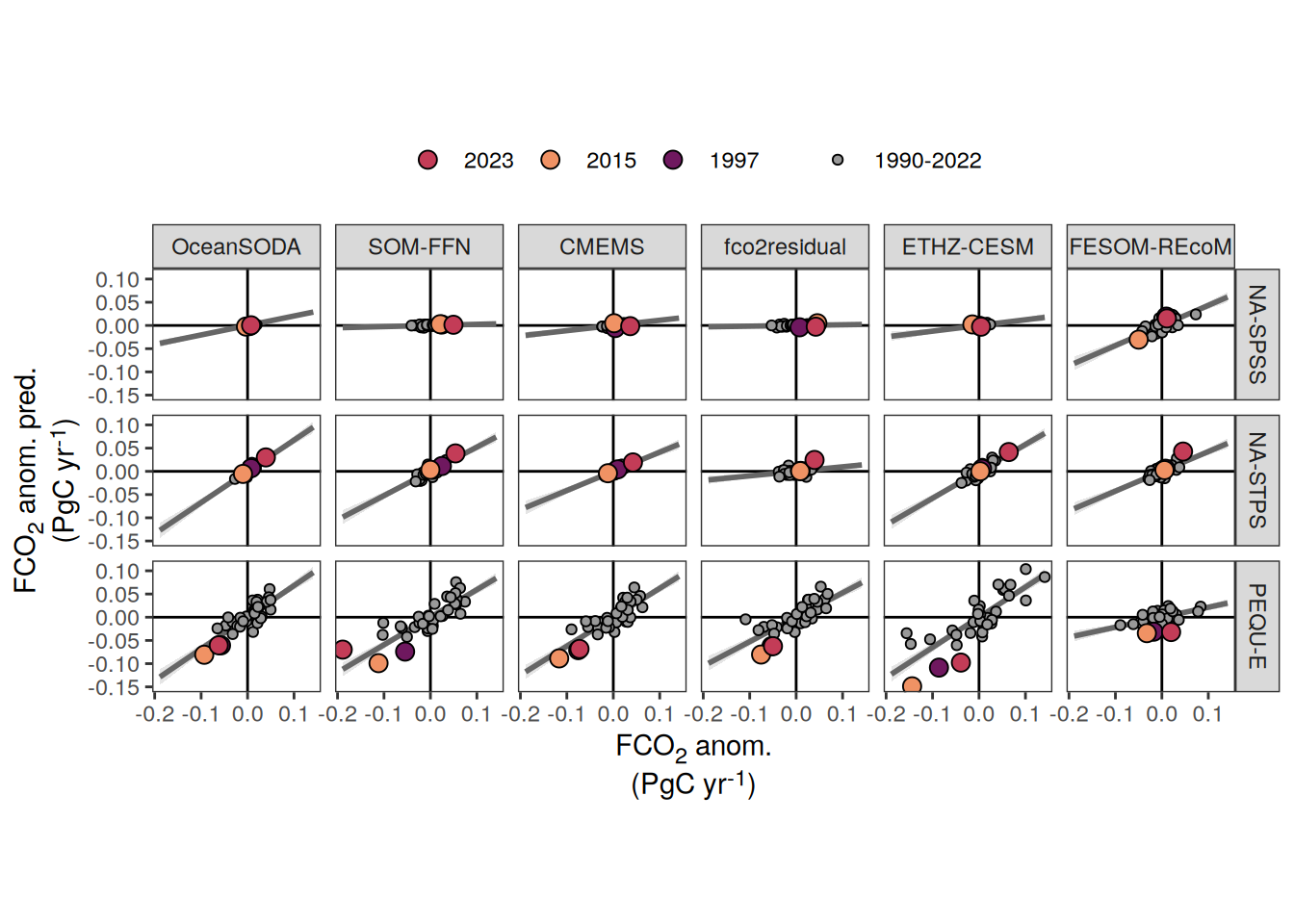
| Version | Author | Date |
|---|---|---|
| b76a7c8 | jens-daniel-mueller | 2025-03-04 |
pco2_product_biome_annual_anomaly_temperature_predict %>%
  select(product, year, biome, fgco2_int, fgco2_predict_int, fgco2_predict_int_biome) %>%
  pivot_longer(contains("predict"),
               values_to = "resid") %>%
  filter(biome %in% c("Global non-polar")) %>%
  ggplot(aes(fgco2_int - resid, fill = name)) +
  geom_vline(xintercept = 0) +
  geom_histogram(binwidth=.05, alpha=.5, position="identity") +
  geom_density(aes(col = name), fill = "transparent") +
  facet_wrap(~ product, scales = "free") +
  theme(
    axis.title.x = element_markdown(),
    axis.title.y = element_markdown(),
    legend.title = element_blank(),
    legend.position = "top"
  )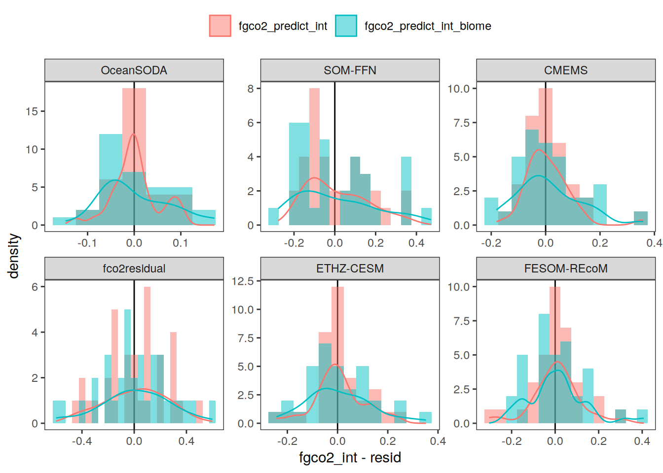
| Version | Author | Date |
|---|---|---|
| b76a7c8 | jens-daniel-mueller | 2025-03-04 |
Monthly anomalies
Absolute
pco2_product_biome_monthly_detrended %>%
  filter(biome == "Global non-polar") %>%
  select(-c(time, fit, value)) %>%
  pivot_wider(values_from = resid) %>%
  pivot_longer(-c(product, year, month, biome, fgco2_int))  %>%
  filter(name == "temperature") %>%
  group_split(name) %>%
  # head(1) %>%
  map(
    ~ ggplot(data = .x,
             aes(value, fgco2_int)) +
      geom_hline(yintercept = 0) +
      geom_point(
        data = . %>% filter(year != 2023),
        aes(col = paste(min(year), max(year), sep = "-")),
        alpha = 0.2
      ) +
      geom_smooth(
        data = . %>% filter(year != 2023),
        aes(col = paste(min(year), max(year), sep = "-")),
        method = "lm",
        se = FALSE,
        fullrange = TRUE
      )  +
      scale_color_grey(name = "") +
      new_scale_color() +
      geom_path(data = . %>% filter(year == 2023),
      aes(col = as.factor(month), group = 1))  +
      geom_point(
        data = . %>% filter(year == 2023),
        aes(fill =  as.factor(month)),
        shape = 21,
        size = 3
      )  +
      scale_color_scico_d(
        palette = "buda",
        guide = guide_legend(reverse = TRUE,
                             order = 1),
        name = paste("Month\nof", 2023)
      ) +
      scale_fill_scico_d(
        palette = "buda",
        guide = guide_legend(reverse = TRUE,
                             order = 1),
        name = paste("Month\nof", 2023)
      ) +
      labs(
        y = labels_breaks("fgco2_int")$i_legend_title,
        x = labels_breaks(unique(.x$name))$i_legend_title
      ) +
      facet_grid(biome ~ product,
                 scales = "free_y") +
      theme(
        axis.title.x = element_markdown(),
        axis.title.y = element_markdown()
      )
  )
[[1]]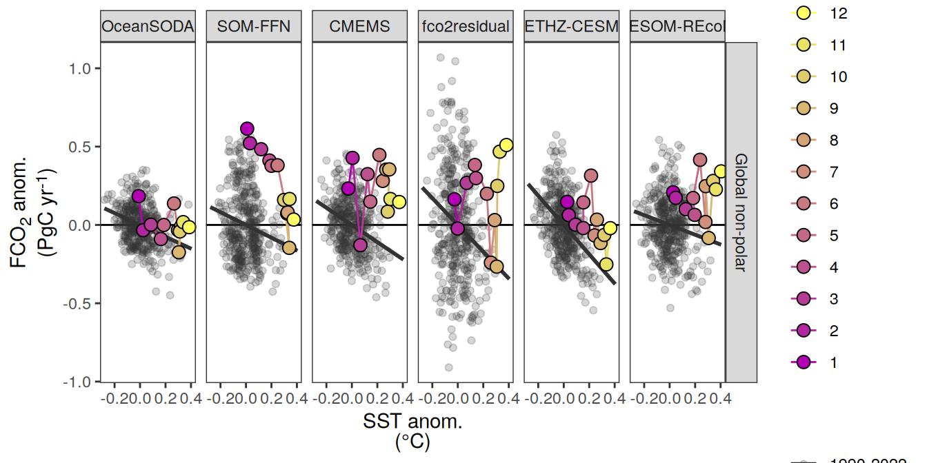
pco2_product_biome_monthly_detrended %>%
  filter(biome %in% key_biomes) %>%
  select(-c(time, fit, value)) %>%
  pivot_wider(values_from = resid) %>%
  pivot_longer(-c(product, year, month, biome, fgco2_int))  %>%
  filter(name == "temperature") %>%
  group_split(name) %>%
  # head(1) %>%
  map(
    ~ ggplot(data = .x,
             aes(value, fgco2_int)) +
      geom_hline(yintercept = 0) +
      geom_point(
        data = . %>% filter(year != 2023),
        aes(col = paste(min(year), max(year), sep = "-")),
        alpha = 0.2
      ) +
      geom_smooth(
        data = . %>% filter(year != 2023),
        aes(col = paste(min(year), max(year), sep = "-")),
        method = "lm",
        se = FALSE,
        fullrange = TRUE
      )  +
      scale_color_grey(name = "") +
      new_scale_color() +
      geom_path(data = . %>% filter(year == 2023),
      aes(col = as.factor(month), group = 1))  +
      geom_point(
        data = . %>% filter(year == 2023),
        aes(fill =  as.factor(month)),
        shape = 21,
        size = 3
      )  +
      scale_color_scico_d(
        palette = "buda",
        guide = guide_legend(reverse = TRUE,
                             order = 1),
        name = paste("Month\nof", 2023)
      ) +
      scale_fill_scico_d(
        palette = "buda",
        guide = guide_legend(reverse = TRUE,
                             order = 1),
        name = paste("Month\nof", 2023)
      ) +
      labs(
        y = labels_breaks("fgco2_int")$i_legend_title,
        x = labels_breaks(unique(.x$name))$i_legend_title
      ) +
      facet_grid(biome ~ product,
                 scales = "free_y") +
      theme(
        axis.title.x = element_markdown(),
        axis.title.y = element_markdown()
      )
  )
[[1]]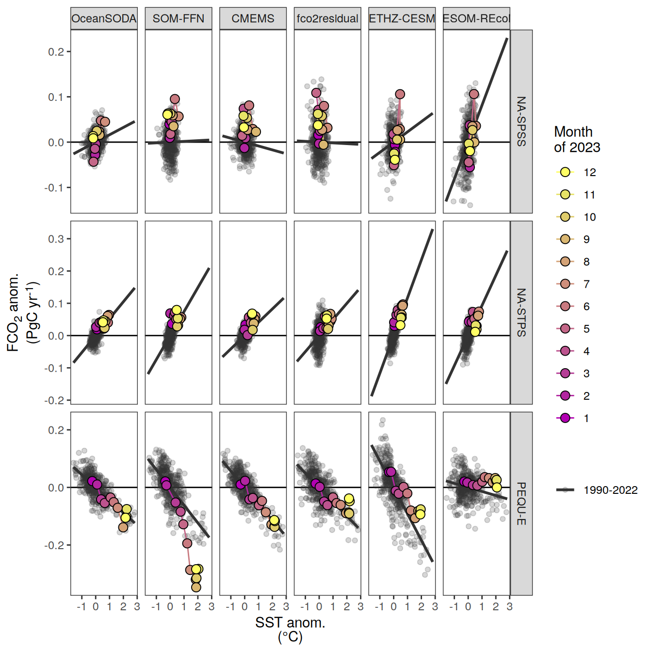
fCO2 decomposition
pco2_product_biome_monthly_fCO2_decomposition %>%
  filter(biome %in% c("Global non-polar",key_biomes)) %>%
  group_split(biome) %>%
  # head(1) %>%
  map(
    ~ p_season(df = .x,
               title  = paste("Anomalies from predicted monthly mean |", .x$biome))
  )
[[1]]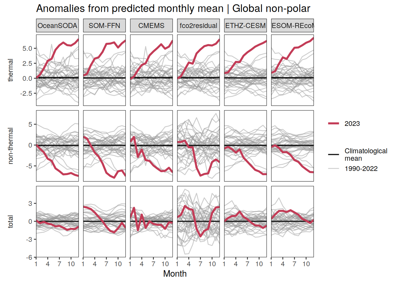
[[2]]
[[3]]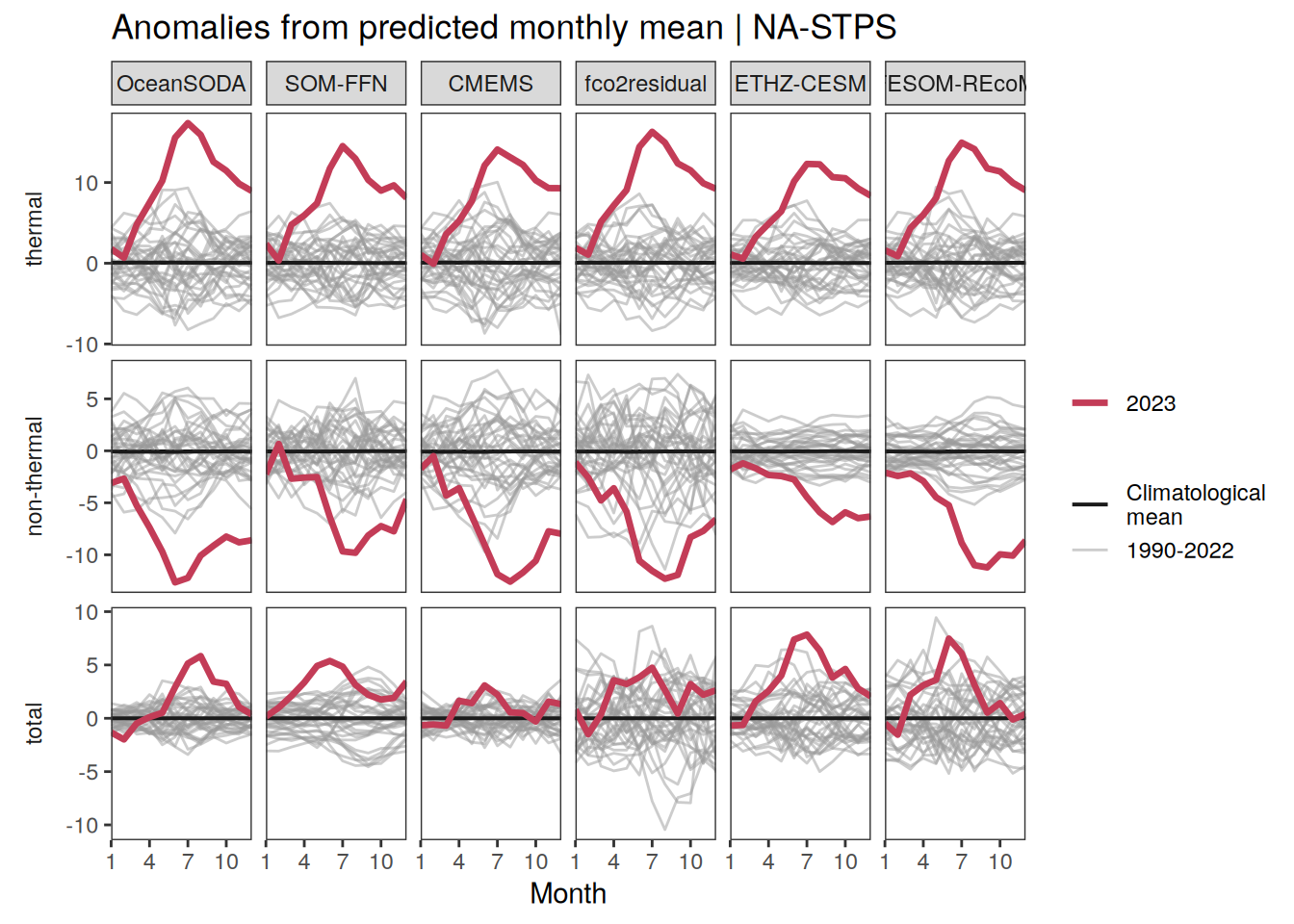
[[4]]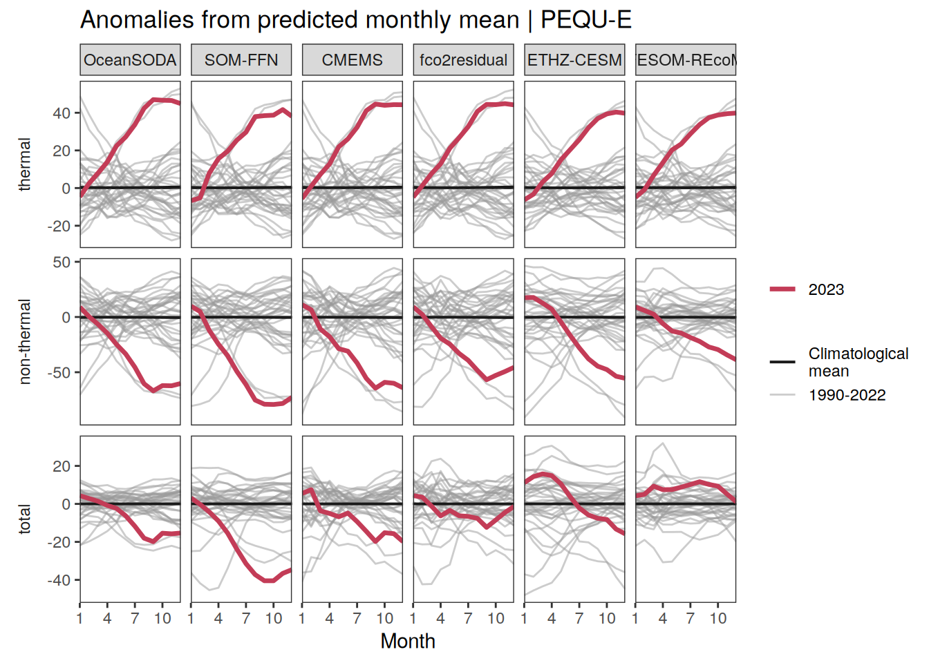
pco2_product_biome_annual_fCO2_decomposition <-
  pco2_product_biome_monthly_fCO2_decomposition %>%
  filter(product %in% pco2_product_list) %>%
  group_by(year, name, biome, product) %>%
  summarise(resid = mean(resid)) %>%
  ungroup()

pco2_product_biome_annual_fCO2_decomposition_ensemble <-
  pco2_product_biome_annual_fCO2_decomposition %>%
  group_by(year, name, biome) %>%
  summarise(resid_sd = sd(resid), resid = mean(resid)) %>%
  ungroup()

pco2_product_biome_annual_fCO2_decomposition_ensemble %>%
  ggplot(aes(year, resid, colour = name)) +
  geom_hline(yintercept = 0) +
  geom_path() +
  facet_wrap( ~ biome)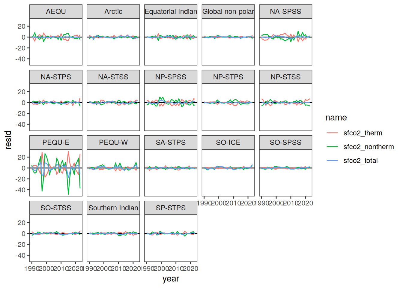
pco2_product_biome_annual_fCO2_decomposition_ensemble %>%
  pivot_wider(values_from = contains("resid")) %>%
  ggplot(aes(resid_sfco2_therm, resid_sfco2_nontherm, col = "observed")) +
  geom_vline(xintercept = 0) +
  geom_hline(yintercept = 0) +
  geom_abline(slope = -1, intercept = 0) +
  geom_smooth(method = "lm", se = FALSE) +
  geom_point(shape = 21) +
  scale_color_muted() +
  facet_wrap( ~ biome, scales = "free")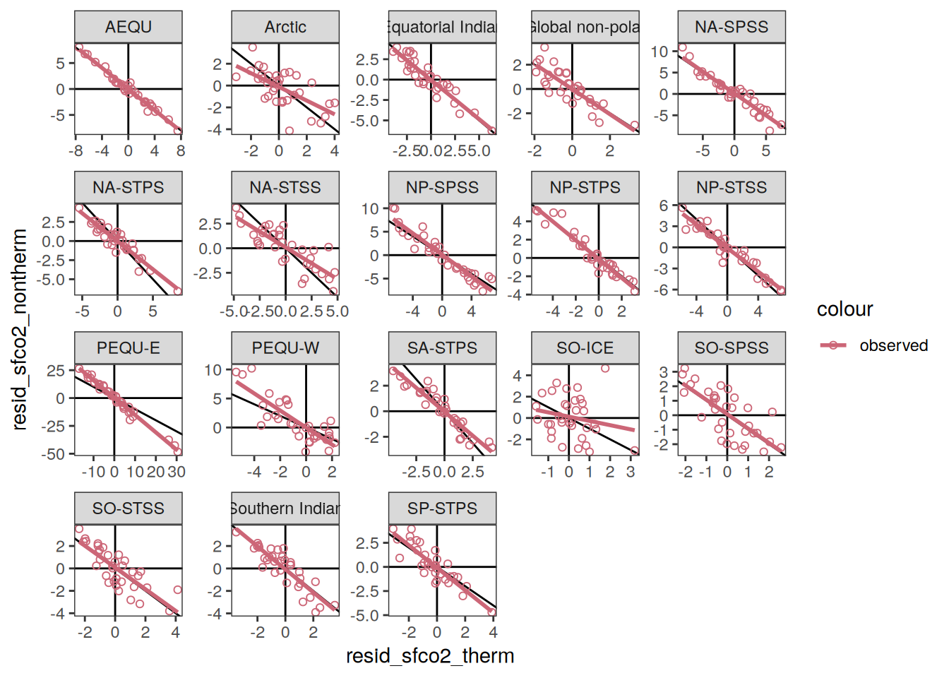
pco2_product_biome_annual_fCO2_decomposition_ensemble %>%
  filter(year == 2023) %>%
  ggplot(aes(name, resid, fill = name)) +
  geom_hline(yintercept = 0) +
  geom_col(col = "grey20") +
  scale_fill_manual(values = c(warm_color, cold_color, "grey80")) +
  labs(y = labels_breaks("sfco2")$i_legend_title) +
  facet_wrap(~ biome, scales = "free_y") +
  theme(
    legend.title = element_blank(),
    axis.text.x = element_blank(),
    axis.ticks.x = element_blank(),
    axis.title.x = element_blank(),
    axis.title.y = element_markdown(),
    legend.position = c(0.9, 0.1)
  )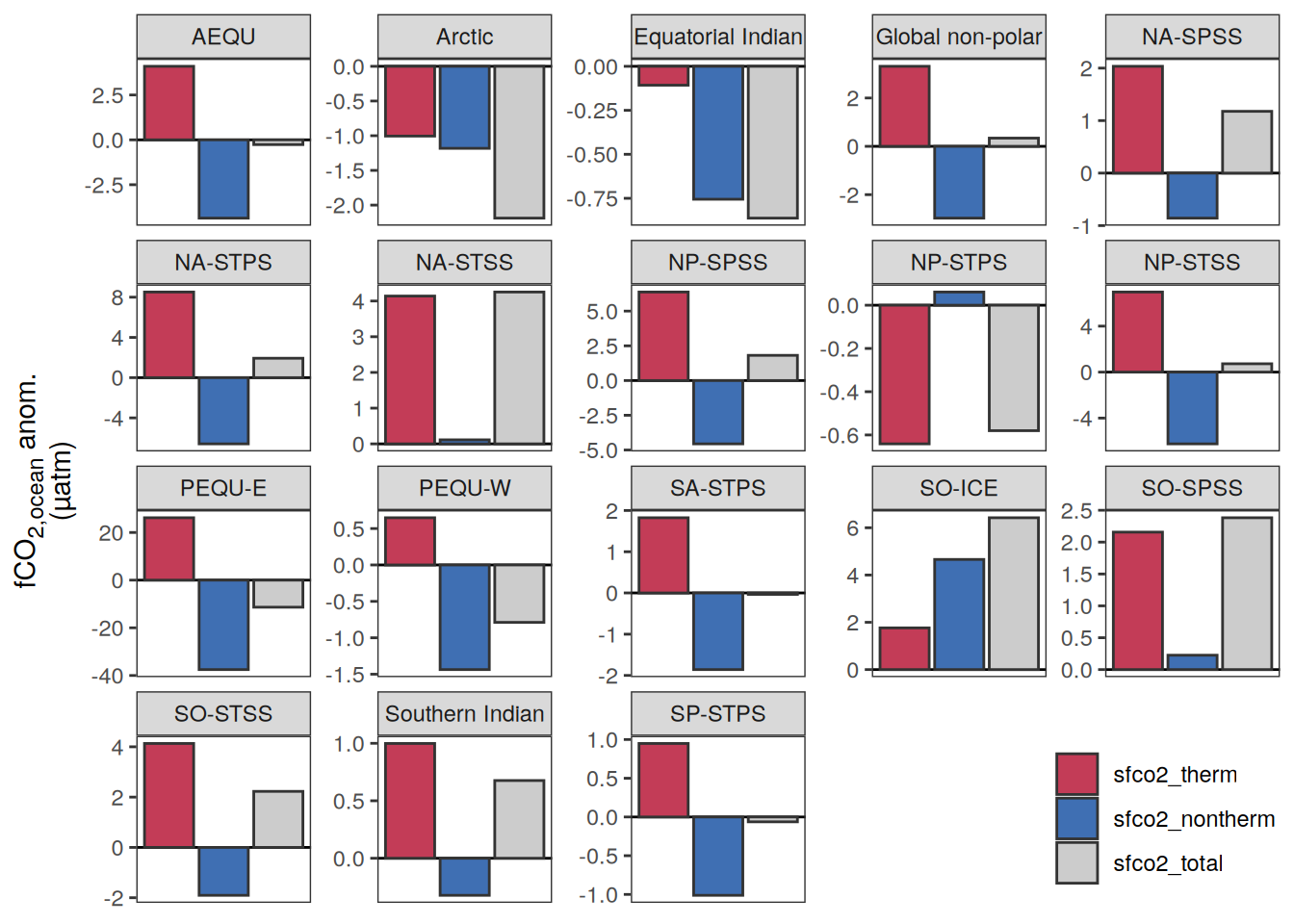
pco2_product_biome_annual_fCO2_decomposition_ensemble %>%
  filter(year == 2023, biome %in% c("PEQU-E", "NA-STPS")) %>%
  mutate(name = case_when(
    name == "sfco2_therm" ~ "thermal",
    name == "sfco2_nontherm" ~ "non-thermal",
    name == "sfco2_total" ~ "total"
  ),
  name = fct_inorder(name)) %>%
  ggplot(aes(name, resid, fill = name)) +
  geom_hline(yintercept = 0) +
  geom_col(col = "grey20") +
  geom_text(
    data = . %>% filter(biome == "NA-STPS"),aes(
    label = name,
    col = name,
    hjust = if_else(sign(resid) > 0, 0, 1),
    y = resid + if_else(sign(resid) > 0, 1, -1)
  ),
  angle = 90,
  fontface = "bold") +
  scale_color_manual(values = c(warm_color, cold_color, "grey20")) +
  scale_fill_manual(values = c(warm_color, cold_color, "grey20")) +
  labs(y = labels_breaks("sfco2")$i_legend_title) +
  scale_y_continuous(breaks = seq(-20, 20, 20)) +
  facet_grid(. ~ fct_rev(biome)) +
  theme_classic() +
  theme(
    legend.title = element_blank(),
    axis.text.x = element_blank(),
    axis.ticks.x = element_blank(),
    axis.title.x = element_blank(),
    axis.title.y = element_markdown(),
    strip.background = element_blank(),
    strip.text = element_text(face = "bold", size = 12),
    axis.line.x = element_blank(),
    legend.position = "none"
  )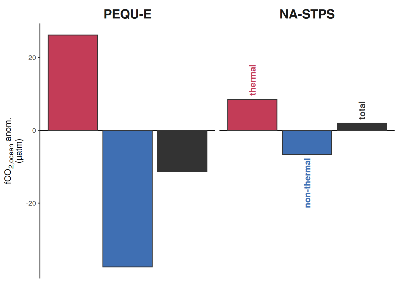
ggsave(width = 4,
       height = 2.5,
       dpi = 1200,
       filename = "../output/biome_annual_fco2_decomposition.pdf")

pco2_product_biome_annual_fCO2_decomposition_ensemble %>%
  filter(year == 2023) %>%
  mutate(name = case_when(
    name == "sfco2_therm" ~ "thermal",
    name == "sfco2_nontherm" ~ "non-thermal",
    name == "sfco2_total" ~ "total"
  ),
  name = fct_inorder(name)) %>%
  ggplot(aes(name, resid, fill = name)) +
  geom_hline(yintercept = 0) +
  geom_col(col = "grey20") +
    geom_linerange(aes(
    name,
    ymin = resid - resid_sd,
    ymax = resid + resid_sd
  ), col = "grey20") +
  scale_color_manual(values = c(warm_color, cold_color, "grey80")) +
  scale_fill_manual(values = c(warm_color, cold_color, "grey80")) +
  geom_point(
    data = pco2_product_biome_annual_fCO2_decomposition %>%
      filter(year == 2023) %>%
      mutate(
        name = case_when(
          name == "sfco2_therm" ~ "thermal",
          name == "sfco2_nontherm" ~ "non-thermal",
          name == "sfco2_total" ~ "total"
        ),
        name = fct_inorder(name)
      ),
    aes(shape = product), col = "grey20"
  ) +
  scale_shape_manual(values = shape_products, name = "fCO2 products") +
  labs(y = labels_breaks("sfco2")$i_legend_title) +
  facet_wrap(. ~ biome, scales = "free_y", ncol = 4) +
  theme(
    legend.title = element_blank(),
    legend.position = c(0.75, 0.1),
    legend.direction = "vertical",
    legend.box = "horizontal",
    axis.text.x = element_blank(),
    axis.ticks.x = element_blank(),
    axis.title.x = element_blank(),
    axis.title.y = element_markdown()
  )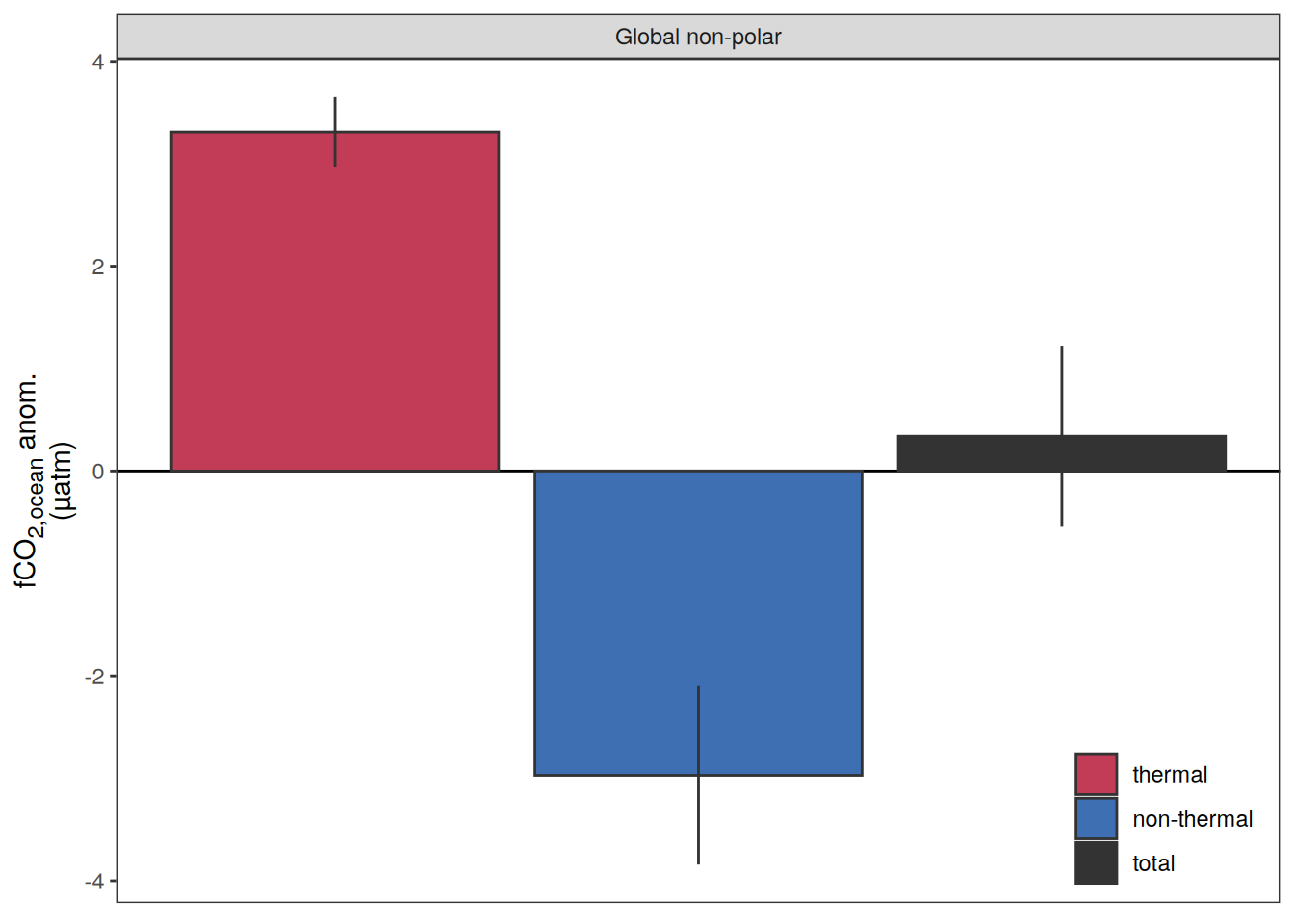
ggsave(width = 7,
       height = 7,
       dpi = 600,
       filename = "../output/biome_annual_fco2_decomposition_all_biomes.pdf")
Flux attribution
Seasonal
pco2_product_biome_annual_flux_attribution_ensemble <-
pco2_product_biome_annual_flux_attribution %>%
      filter(product %in% pco2_product_list) %>%
      group_by(biome, name) %>%
      summarise(
        resid_sd = sd(resid),
        resid = mean(resid)) %>%
      ungroup()


pco2_product_biome_annual_flux_attribution_ensemble %>%
  filter(biome %in% c("Global non-polar", key_biomes)) %>%
  ggplot() +
  geom_hline(yintercept = 0) +
  geom_col(aes("", resid), fill = "grey90", col = "grey20") +
  geom_point(
    data = pco2_product_biome_annual_flux_attribution %>%
      filter(biome %in% c("Global non-polar", key_biomes)),
    aes("", resid, fill = product),
    shape = 21
  ) +
  scale_fill_manual(values = color_products) +
  scale_y_continuous(breaks = seq(-10, 10, 0.1)) +
  labs(y = labels_breaks(unique("fgco2"))$i_legend_title)+
  facet_grid(
    biome ~ name,
    labeller = labeller(name = x_axis_labels),
    scales = "free_y",
    space = "free_y",
    switch = "x"
  ) +
  theme(
    legend.title = element_blank(),
    axis.text.x = element_blank(),
    axis.ticks.x = element_blank(),
    axis.title.x = element_blank(),
    axis.title.y = element_markdown(),
    strip.text.x.bottom = element_markdown(),
    strip.placement = "outside",
    strip.background.x = element_blank(),
    legend.position = "top"
  )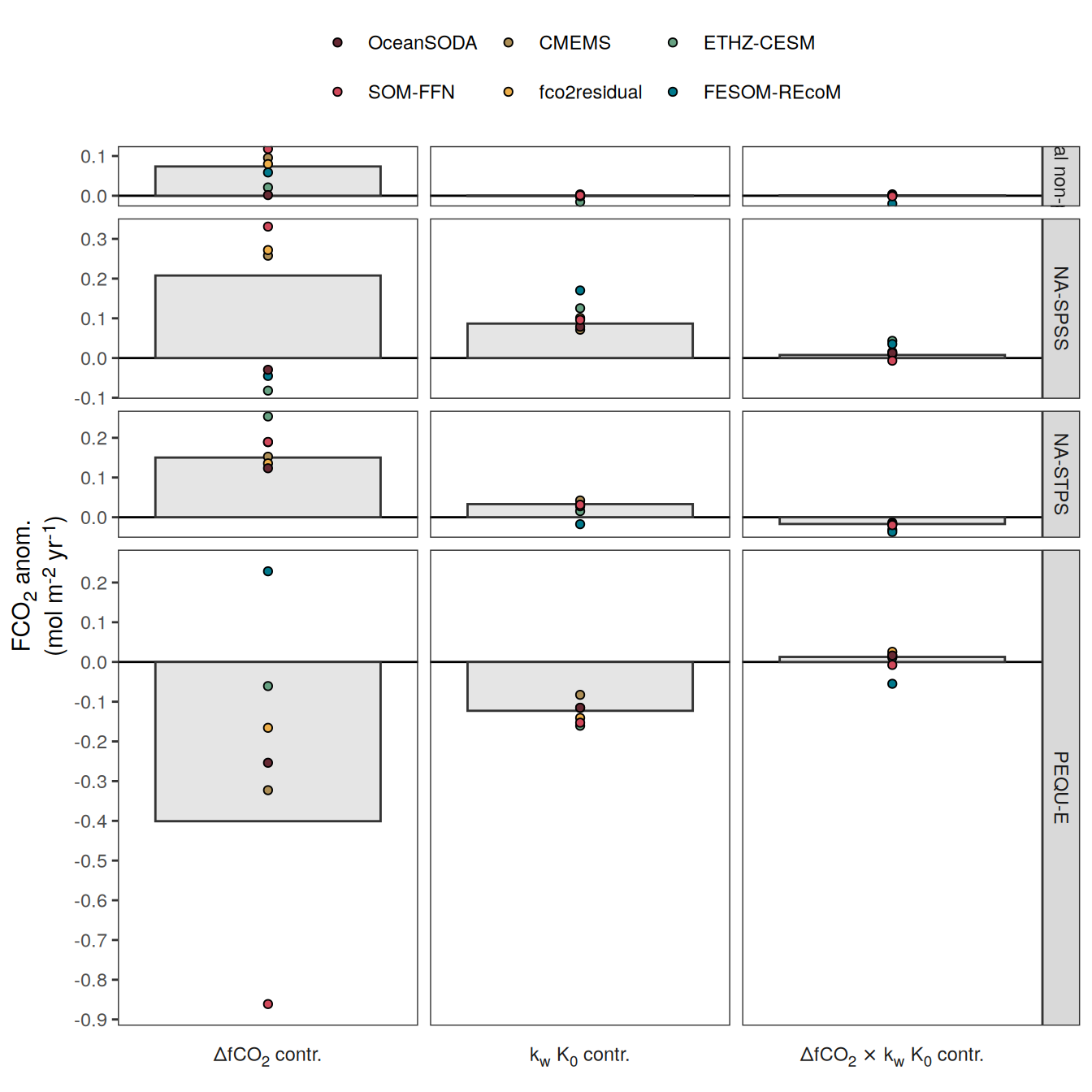
pco2_product_biome_annual_flux_attribution_ensemble %>%
  ggplot(aes(name, resid, fill = name)) +
  geom_hline(yintercept = 0) +
  geom_col(aes(name, resid, fill = name), col = "grey20") +
  geom_linerange(aes(
    ymin = resid - resid_sd,
    ymax = resid + resid_sd
  ), col = "grey20") +
  scale_fill_bright(labels = x_axis_labels) +
  geom_point(
    data = pco2_product_biome_annual_flux_attribution %>%
      filter(product %in% pco2_product_list),
    aes(shape = product), col = "grey20"
  ) +
  scale_shape_manual(values = shape_products, name = "fCO2 products") +
  labs(y = labels_breaks(unique("fgco2"))$i_legend_title) +
  facet_wrap( ~ biome, scales = "free_y", ncol = 4) +
  theme(
    legend.title = element_blank(),
    legend.text = element_markdown(),
    legend.position = c(0.75, 0.1),
    legend.direction = "vertical",
    legend.box = "horizontal",
    axis.text.x = element_blank(),
    axis.ticks.x = element_blank(),
    axis.title.x = element_blank(),
    axis.title.y = element_markdown()
  )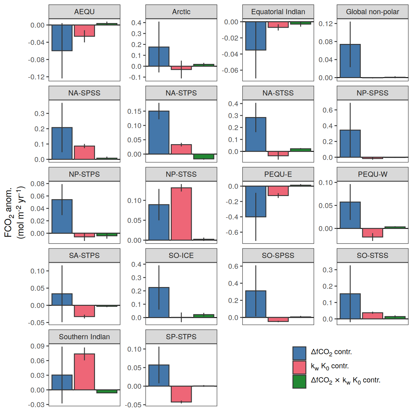
ggsave(width = 7,
       height = 7,
       dpi = 600,
       filename = "../output/biome_annual_flux_attribution_all_biomes.pdf")


ggplot() +
  geom_hline(yintercept = 0) +
  geom_col(
    data = pco2_product_biome_annual_flux_attribution %>%
      filter(biome %in% c("Global non-polar", key_biomes)),
    aes("", resid, fill = product),
    position = position_dodge(width = 1),
    alpha = 0.5, col = "grey30"
  ) +
  geom_point(
    data = pco2_product_biome_monthly_flux_attribution %>%
      filter(year == 2023,
             biome %in% c("Global non-polar", key_biomes)),
    aes("", resid, fill = product),
    position = position_dodge(width = 1),
    shape = 21, alpha = 0.5, col = "grey30"
  ) +
  scale_fill_manual(values = color_products) +
  # scale_color_manual(values = color_products) +
  scale_y_continuous(breaks = seq(-10,10,0.2)) +
  labs(y = labels_breaks(unique("fgco2"))$i_legend_title) +
  facet_grid(biome ~ name,
             labeller = labeller(name = x_axis_labels),
                          scales = "free_y",
             space = "free_y",
             switch = "x") +
  theme(
    legend.title = element_blank(),
    axis.text.x = element_blank(),
    axis.ticks.x = element_blank(),
    axis.title.x = element_blank(),
    axis.title.y = element_markdown(),
    strip.text.x.bottom = element_markdown(),
    strip.placement = "outside",
    strip.background.x = element_blank(),
    legend.position = "top"
  )
pco2_product_biome_monthly_flux_attribution %>%
  filter(year == 2023,
         biome %in% c("Global non-polar", key_biomes)) %>%
  ggplot() +
  geom_hline(yintercept = 0) +
  geom_path(
    aes(month, resid, col = product)
  ) +
  geom_point(
    aes(month, resid, fill = product),
    shape = 21,
    alpha = 0.5,
    col = "grey30"
  ) +
  scale_fill_manual(values = color_products) +
  scale_color_manual(values = color_products) +
  scale_y_continuous(breaks = seq(-10,10,0.2)) +
  scale_x_continuous(position = "top", breaks = seq(1,12,3)) +
  labs(y = labels_breaks(unique("fgco2"))$i_legend_title) +
  facet_grid(biome ~ name,
             labeller = labeller(name = x_axis_labels),
             scales = "free_y",
             space = "free_y",
             switch = "x") +
  theme(
    legend.title = element_blank(),
    axis.title.y = element_markdown(),
    strip.text.x.bottom = element_markdown(),
    strip.placement = "outside",
    strip.background.x = element_blank(),
    legend.position = "top"
  )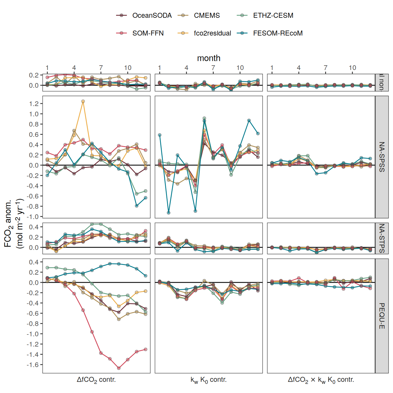
pco2_product_biome_monthly_flux_attribution %>%
  filter(biome %in% c("Global non-polar", key_biomes)) %>%
  group_split(biome) %>%
  # head(1) %>%
  map(
    ~ p_season(
      df = .x,
      title  = paste("Anomalies from predicted monthly mean |", .x$biome)
    ) +
      facet_grid(
        name ~ product,
        labeller = labeller(name = x_axis_labels),
        switch = "y"
      ) +
      theme(
        strip.text.y.left = element_markdown(),
        strip.placement = "outside",
        strip.background.y = element_blank(),
        axis.title.y = element_blank(),
        legend.title = element_blank()
      )
  )
[[1]]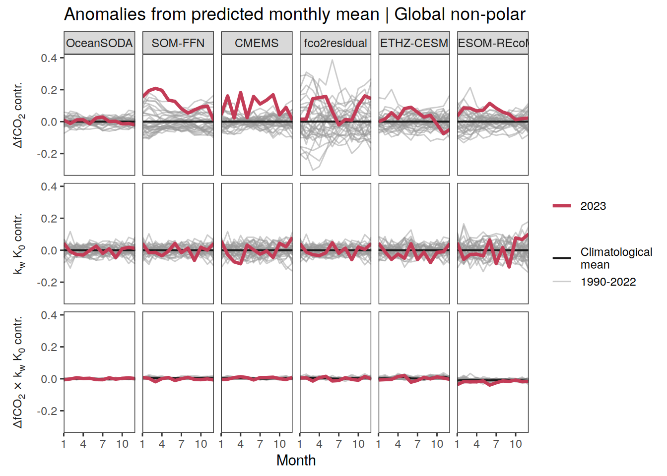
[[2]]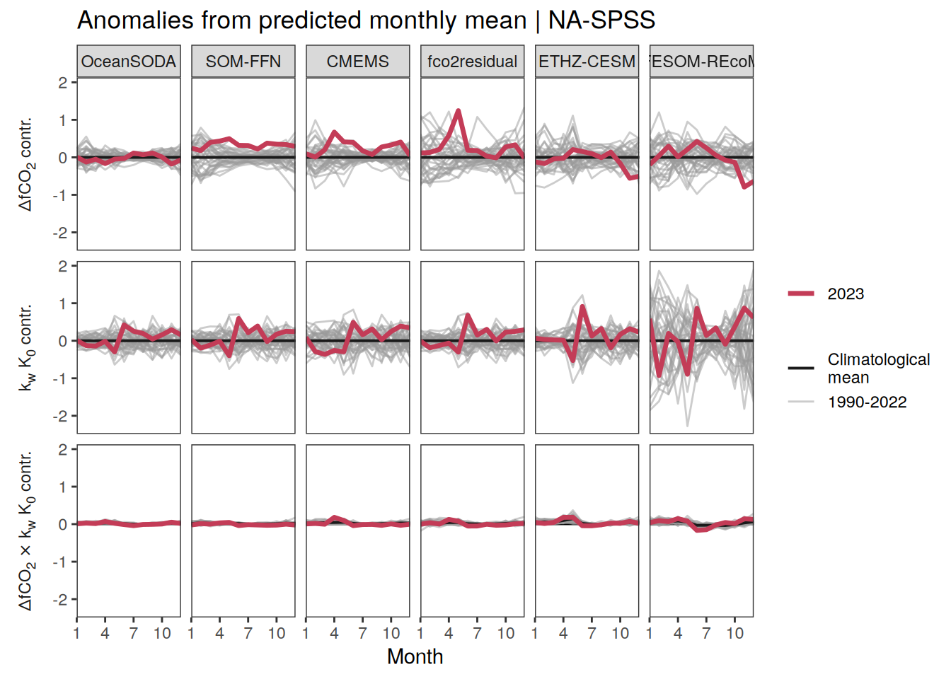
[[3]]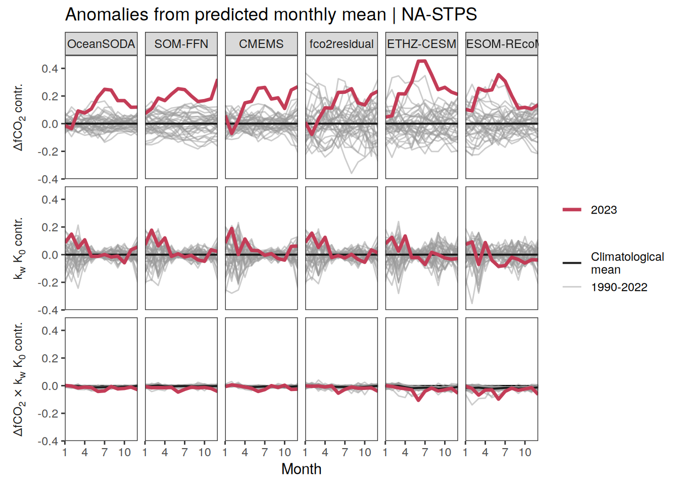
[[4]]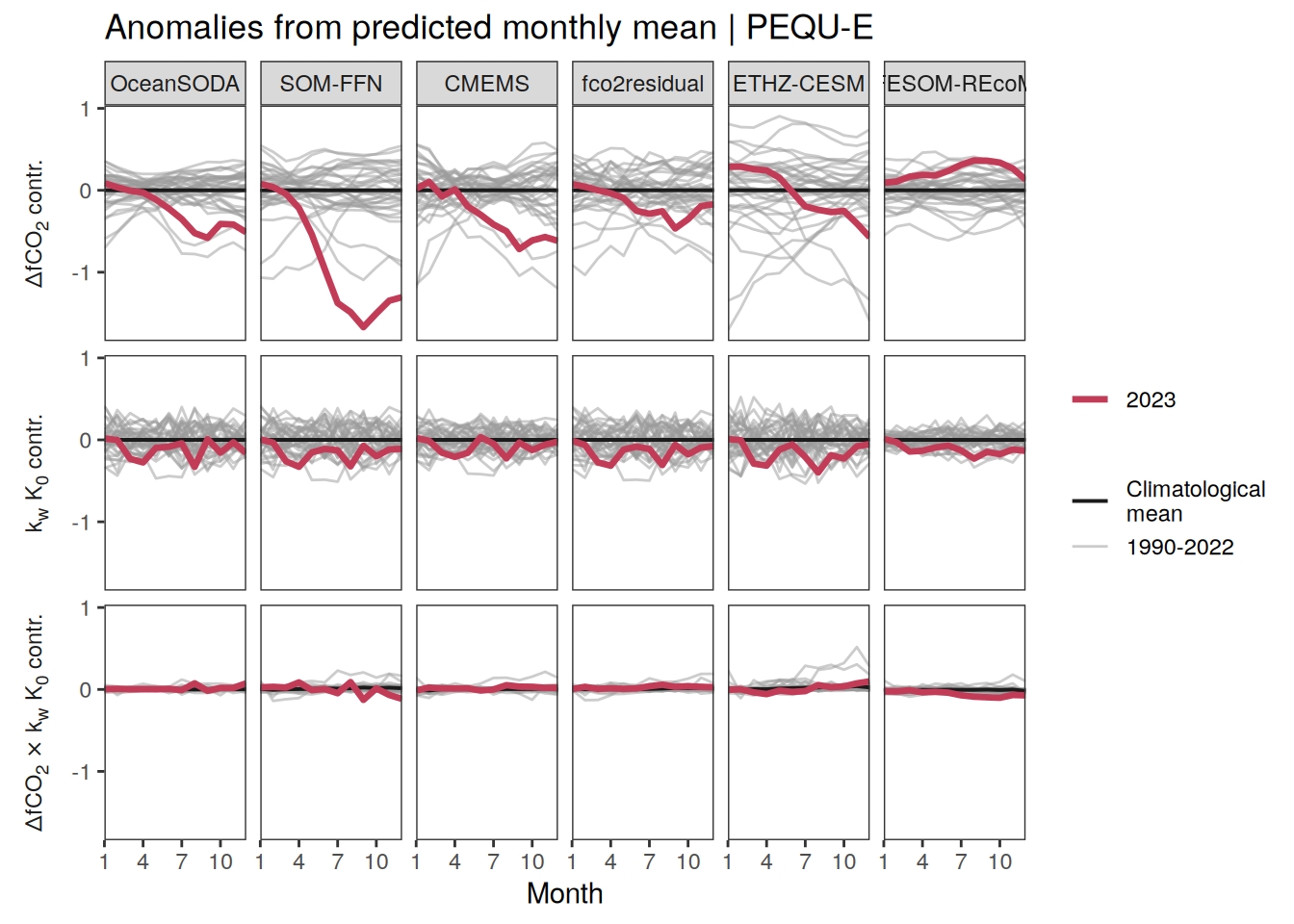
Annual
# pco2_product_biome_annual_flux_attribution <-
# full_join(
# pco2_product_biome_annual_flux_attribution %>%
#   filter(year == 2023) %>%
#   select(-year),
# pco2_product_biome_annual_flux_attribution %>%
#   filter(year != 2023) %>%
#   group_by(product, biome, name) %>%
#   summarise(resid_mean = mean(abs(resid))) %>%
#   ungroup())

pco2_product_biome_annual_flux_attribution %>%
  filter(biome %in% c("Global non-polar", key_biomes)) %>%
  group_split(biome) %>%
  # head(1) %>%
  map(
    ~ ggplot(data = .x) +
      geom_col(aes("x", resid, fill = product),
               position = "dodge2") +
      scale_fill_manual(values = color_products) +
      geom_col(
        aes(
          "x",
          resid_mean * sign(resid),
          group = product,
          col = paste0("Mean\nexcl.",2023)
        ),
        position = "dodge2",
        fill = "transparent"
      ) +
      labs(y = labels_breaks(unique("fgco2"))$i_legend_title,
           title = .x$biome) +
      facet_grid(
        .~name,
        labeller = labeller(name = x_axis_labels),
        switch = "x"
      ) +
      scale_color_grey() +
      theme(
        legend.title = element_blank(),
        axis.text.x = element_blank(),
        axis.ticks.x = element_blank(),
        axis.title.x = element_blank(),
        axis.title.y = element_markdown(),
        strip.text.x.bottom = element_markdown(),
        strip.placement = "outside",
        strip.background.x = element_blank(),
        legend.position = "top"
      )
  )
[[1]]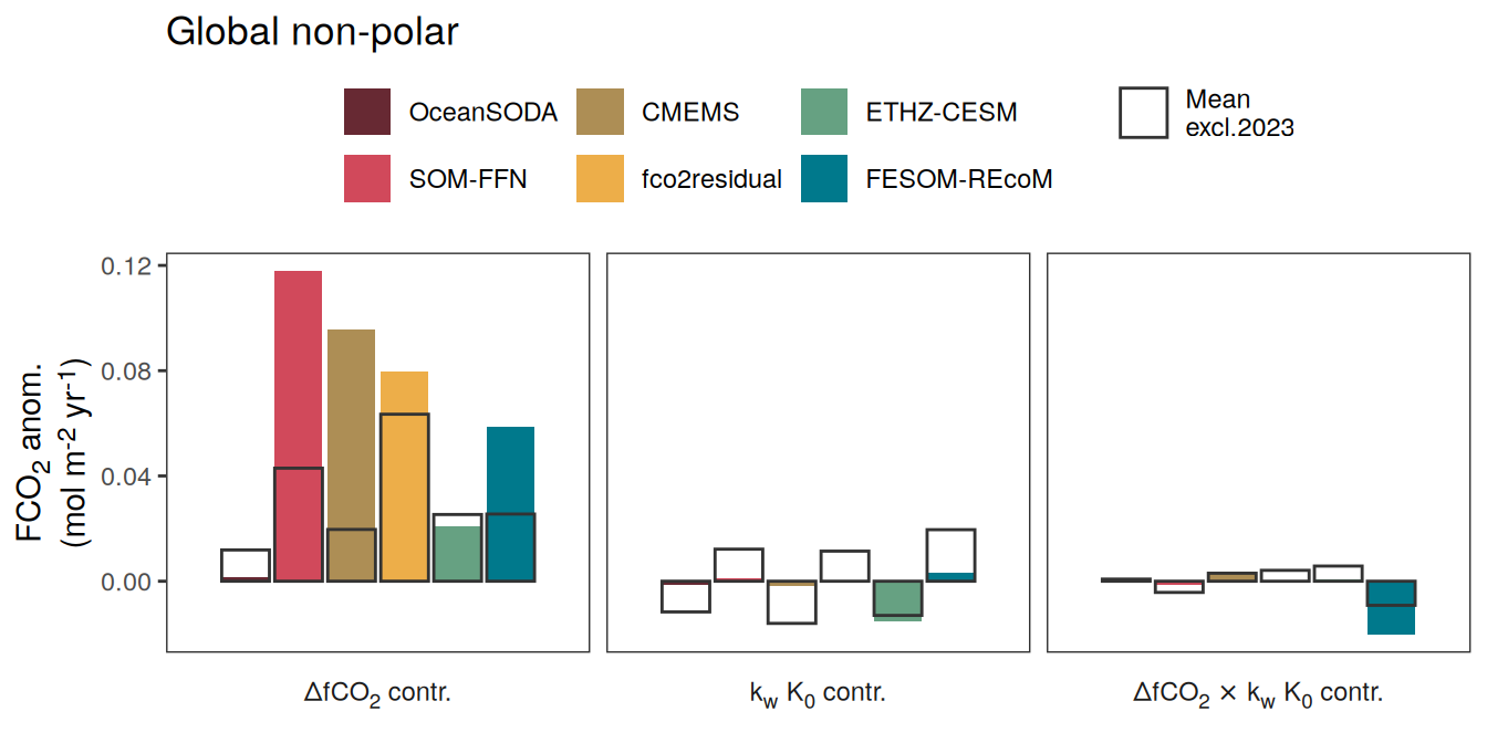
[[2]]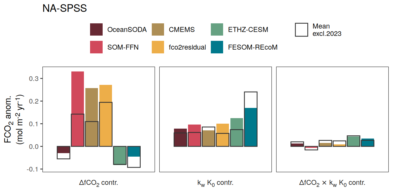
[[3]]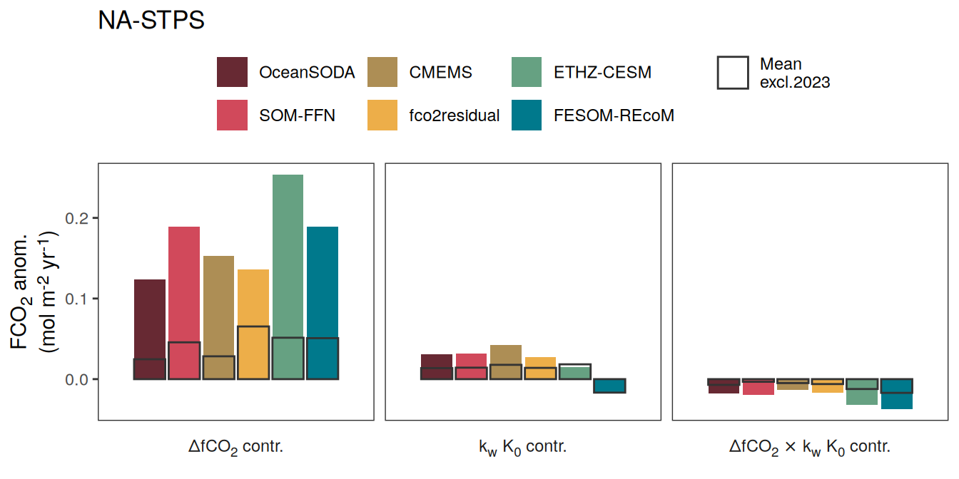
[[4]]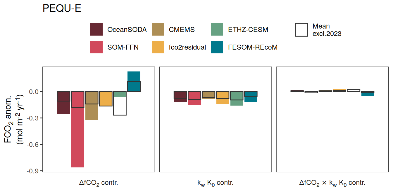
Merged seasonality plots
pco2_product_biome_monthly_detrended %>%
  filter(product %in% pco2_product_list) %>%
  group_by(year, month, biome, name) %>%
  summarise(across(where(is.numeric), mean)) %>%
  ungroup() %>%
  filter(name %in% c("temperature", "fgco2"), biome %in% key_biomes,
         year != 2023) %>%
  group_by(month, biome, name) %>%
  summarise(resid_sd = sd(resid)) %>%
  ungroup() %>%
  ggplot(aes(month, resid_sd)) +
  geom_path() +
  facet_grid(name ~ biome, scales = "free_y")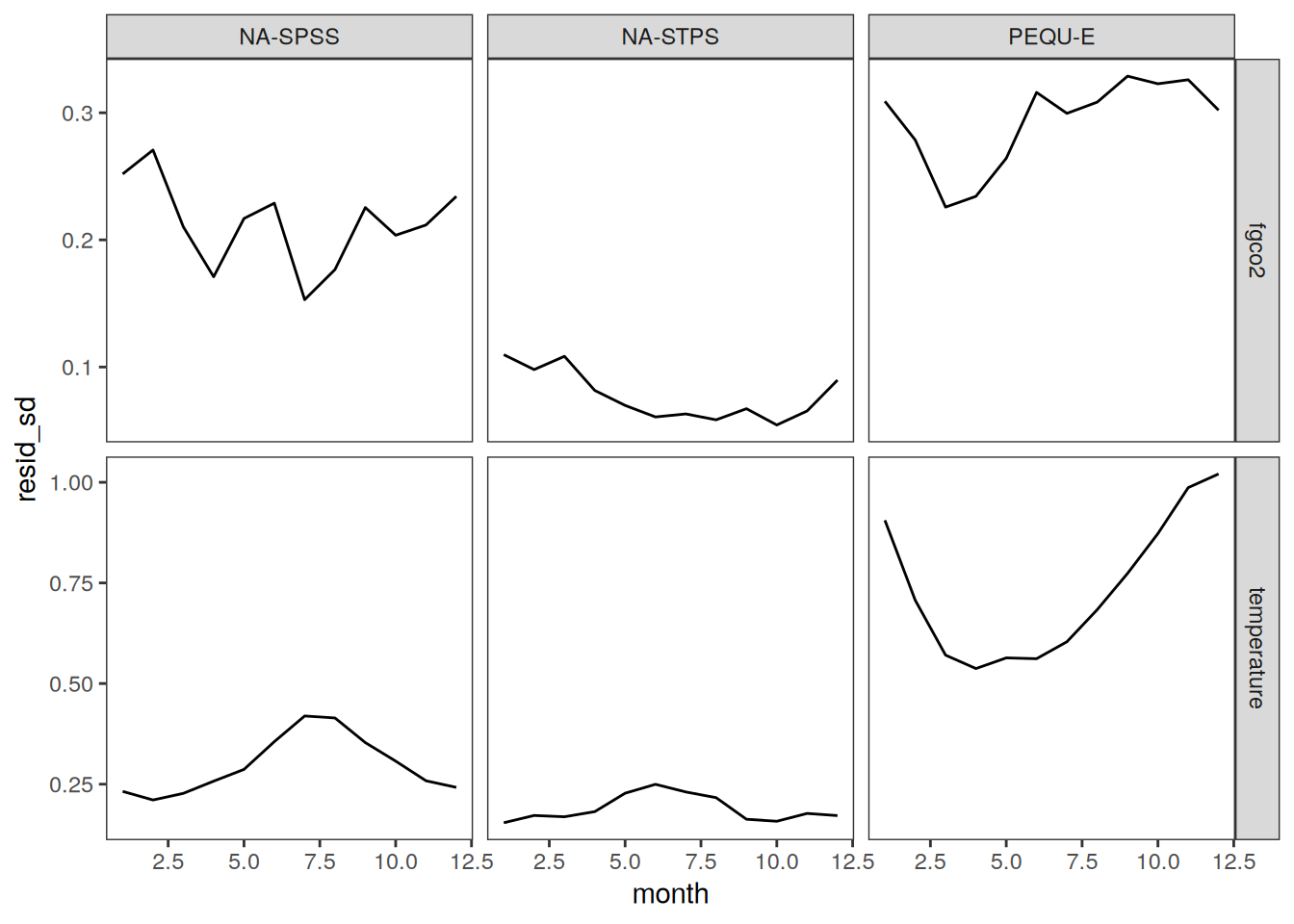
pco2_product_biome_monthly_detrended %>%
  filter(product %in% pco2_product_list) %>%
  group_by(year, month, biome, name) %>%
  summarise(across(where(is.numeric), mean)) %>%
  ungroup() %>%
  filter(name %in% c("temperature", "fgco2"), biome %in% key_biomes) %>%
  p_season(dim_col = "biome") +
  theme(axis.title.x = element_blank(),
        axis.text.x = element_blank(),
        legend.position = "none") +
  new_scale_color() +
  scale_color_manual(values = warm_cool_gradient[15]) +
  geom_path(
    data = pco2_product_biome_monthly_detrended %>%
      filter(
        product %in% gobm_product_list,
        year == 2023,
        name %in% c("temperature", "fgco2"),
        biome %in% key_biomes
      ) %>%
      group_by(year, month, biome, name) %>%
      summarise(across(where(is.numeric), mean)) %>%
      ungroup(),
    aes(month, resid, col = "2023\nGOBM mean")
  )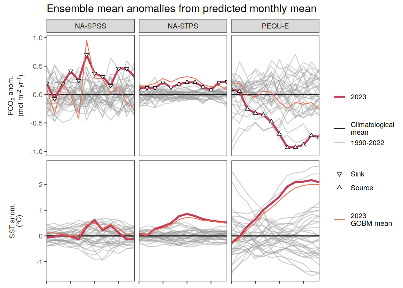
ggsave(width = 9,
       height = 4,
       dpi = 600,
       filename = "../output/Fig4_ab.pdf")


pco2_product_biome_monthly_detrended %>%
  filter(product %in% pco2_product_list) %>%
  group_by(year, month, biome, name) %>%
  summarise(across(where(is.numeric), mean)) %>%
  ungroup() %>%
  filter(name %in% c("temperature", "fgco2"), biome %in% key_biomes[2:3]) %>%
  p_season(dim_col = "biome",
           title = "Ensemble mean anomalies from predicted monthly mean") +
  theme(axis.title.x = element_blank(), axis.text.x = element_blank()) +
  new_scale_color() +
  scale_color_manual(values = warm_cool_gradient[15]) +
  geom_path(
    data = pco2_product_biome_monthly_detrended %>%
      filter(
        product %in% gobm_product_list,
        year == 2023,
        name %in% c("temperature", "fgco2"),
        biome %in% key_biomes[2:3]
      ) %>%
      group_by(year, month, biome, name) %>%
      summarise(across(where(is.numeric), mean)) %>%
      ungroup(),
    aes(month, resid, col = "2023\nGOBM mean")
  )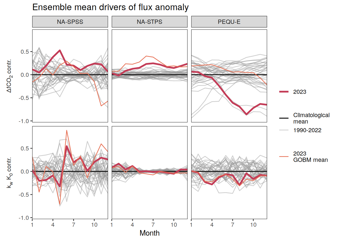
ggsave(width = 8,
       height = 4,
       dpi = 1200,
       filename = "../output/biome_seasonal_anomaly_fgco2_sst_ensemble_mean_pco2_products_2_biomes.pdf")

pco2_product_biome_monthly_flux_attribution %>%
  filter(product %in% pco2_product_list) %>%
  group_by(year, month, biome, name) %>%
  summarise(across(where(is.numeric), mean)) %>%
  ungroup() %>%
  filter(name %in% c("resid_fgco2_dfco2", "resid_fgco2_kw_sol"),
         biome %in% key_biomes) %>%
  p_season(dim_col = "biome",
           title = "Ensemble mean drivers of flux anomaly",
           scales = "fixed") +
  new_scale_color() +
  scale_color_manual(values = warm_cool_gradient[15]) +
  geom_path(
    data = pco2_product_biome_monthly_flux_attribution %>%
      filter(
        product %in% gobm_product_list,
        year == 2023,
        name %in% c("resid_fgco2_dfco2", "resid_fgco2_kw_sol"),
        biome %in% key_biomes
      ) %>%
      group_by(year, month, biome, name) %>%
      summarise(across(where(is.numeric), mean)) %>%
      ungroup(),
    aes(month, resid, col = "2023\nGOBM mean")
  )
ggsave(width = 9,
       height = 4,
       dpi = 600,
       filename = "../output/biome_seasonal_anomaly_fgco2_attribution_ensemble_mean_pco2_products.pdf")

pco2_product_biome_monthly_fCO2_decomposition %>%
  filter(product %in% pco2_product_list) %>%
  group_by(year, month, biome, name) %>%
  summarise(across(where(is.numeric), mean)) %>%
  ungroup() %>%
  filter(name %in% c("sfco2_nontherm", "sfco2_therm", "sfco2_total"),
         biome %in% c("Global non-polar", key_biomes)) %>%
  p_season(dim_col = "biome",
title = "Ensemble mean decomposition of fCO2 anomaly") 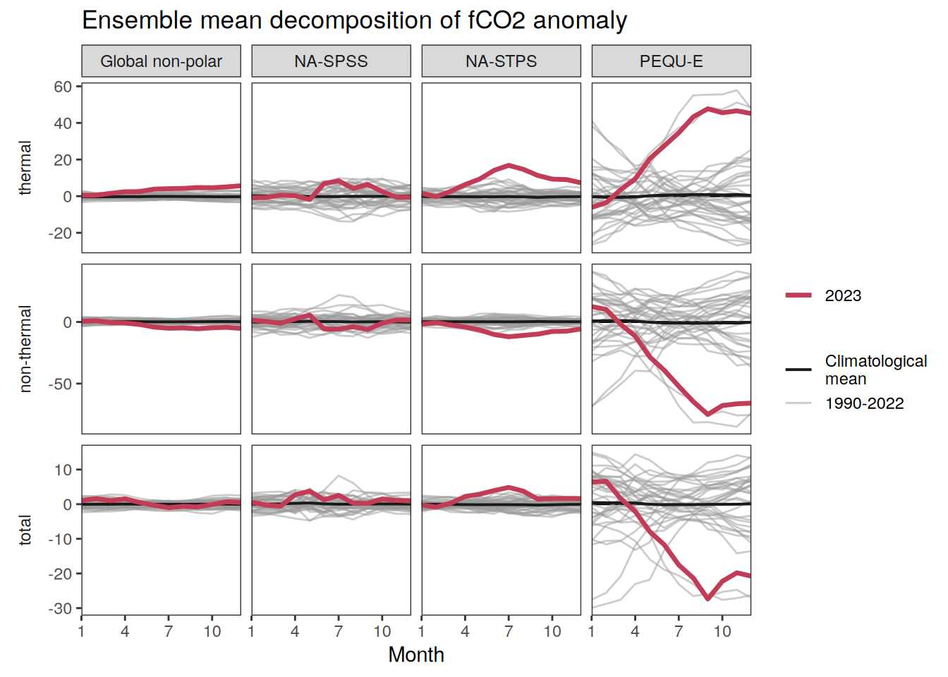
| Version | Author | Date |
|---|---|---|
| 265b0a8 | jens-daniel-mueller | 2025-06-06 |
ggsave(width = 9,
       height = 4,
       dpi = 600,
       filename = "../output/biome_seasonal_anomaly_fco2_decomposition_ensemble_mean_pco2_products.pdf")
pco2_product_biome_monthly_detrended %>%
filter(year == 2023,
name %in% c("temperature", "fgco2"),
biome %in% c("Global non-polar", key_biomes)) %>%
ggplot(aes(month, resid)) +
geom_hline(yintercept = 0, linewidth = 0.5) +
geom_path(aes(col = product)) +
scale_color_manual(values = color_products) +
scale_x_continuous(breaks = seq(1, 12, 3), expand = c(0, 0)) +
labs(x = "Month",
title = "Anomalies from predicted monthly mean") +
facet_grid(
name ~ biome,
scales = "free_y",
labeller = labeller(name = x_axis_labels),
switch = "y"
) +
theme(
strip.text.y.left = element_markdown(),
strip.placement = "outside",
strip.background.y = element_blank(),
axis.title.y = element_blank(),
legend.title = element_blank()
)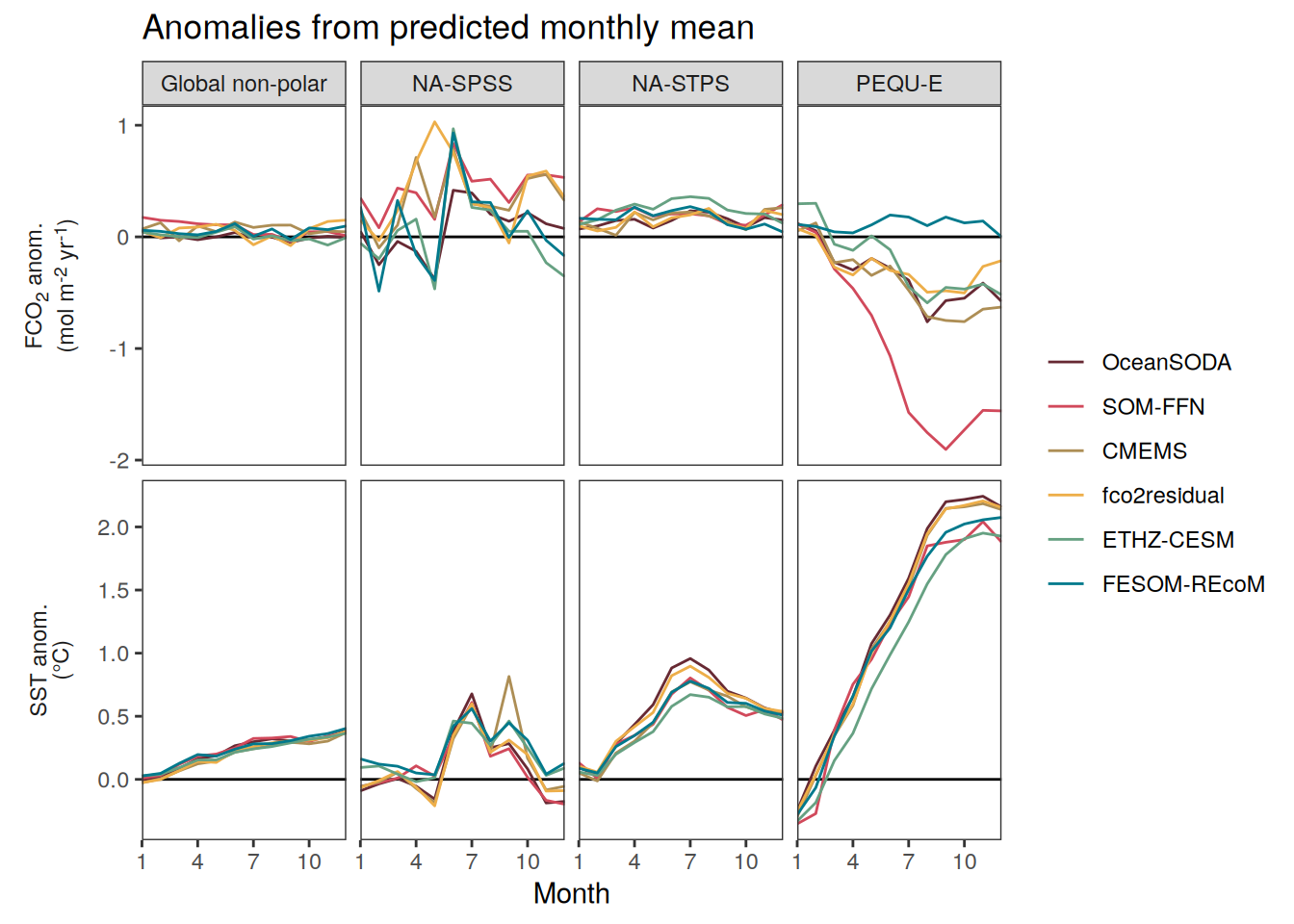
ggsave(width = 9,
       height = 3,
       dpi = 600,
       filename = "../output/biome_seasonal_anomaly_fgco2_sst_all_products.pdf")

pco2_product_biome_monthly_flux_attribution %>%
  filter(year == 2023,
         name %in% c("resid_fgco2_dfco2", "resid_fgco2_kw_sol"),
         biome %in% c("Global non-polar", key_biomes)) %>%
  ggplot(aes(month, resid)) +
  geom_hline(yintercept = 0, linewidth = 0.5) +
  geom_path(aes(col = product)) +
  scale_color_manual(values = color_products) +
  scale_x_continuous(breaks = seq(1, 12, 3), expand = c(0, 0)) +
  labs(x = "Month",
       title = "Drivers of flux anomaly") +
  facet_grid(
    name ~ biome,
    scales = "fixed",
    labeller = labeller(name = x_axis_labels),
    switch = "y"
  ) +
  theme(
    strip.text.y.left = element_markdown(),
    strip.placement = "outside",
    strip.background.y = element_blank(),
    axis.title.y = element_blank(),
    legend.title = element_blank()
  )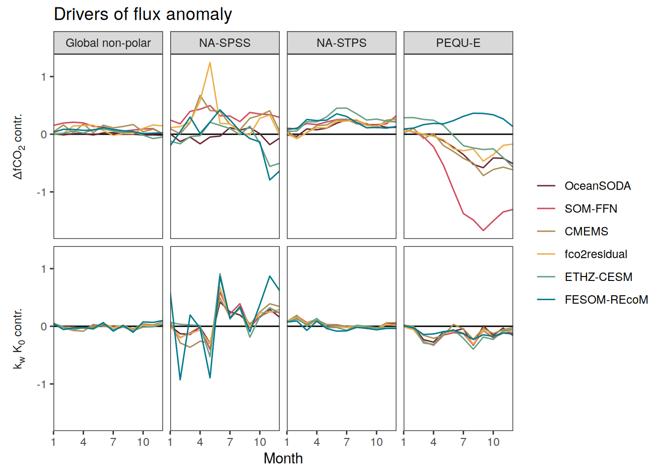
ggsave(width = 9,
       height = 3,
       dpi = 600,
       filename = "../output/biome_seasonal_anomaly_fgco2_attribution_all_products.pdf")

pco2_product_biome_monthly_fCO2_decomposition %>%
  filter(year == 2023,
         name %in% c("sfco2_nontherm", "sfco2_therm", "sfco2_total"),
         biome %in% c("Global non-polar", key_biomes)) %>%
  ggplot(aes(month, resid)) +
  geom_hline(yintercept = 0, linewidth = 0.5) +
  geom_path(aes(col = product)) +
  scale_color_manual(values = color_products) +
  scale_x_continuous(breaks = seq(1, 12, 3), expand = c(0, 0)) +
  labs(x = "Month",
       title = "Decomposition of fCO2 anomaly") +
  facet_grid(
    name ~ biome,
    scales = "free_y",
    labeller = labeller(name = x_axis_labels),
    switch = "y"
  ) +
  theme(
    strip.text.y.left = element_markdown(),
    strip.placement = "outside",
    strip.background.y = element_blank(),
    axis.title.y = element_blank(),
    legend.title = element_blank()
  )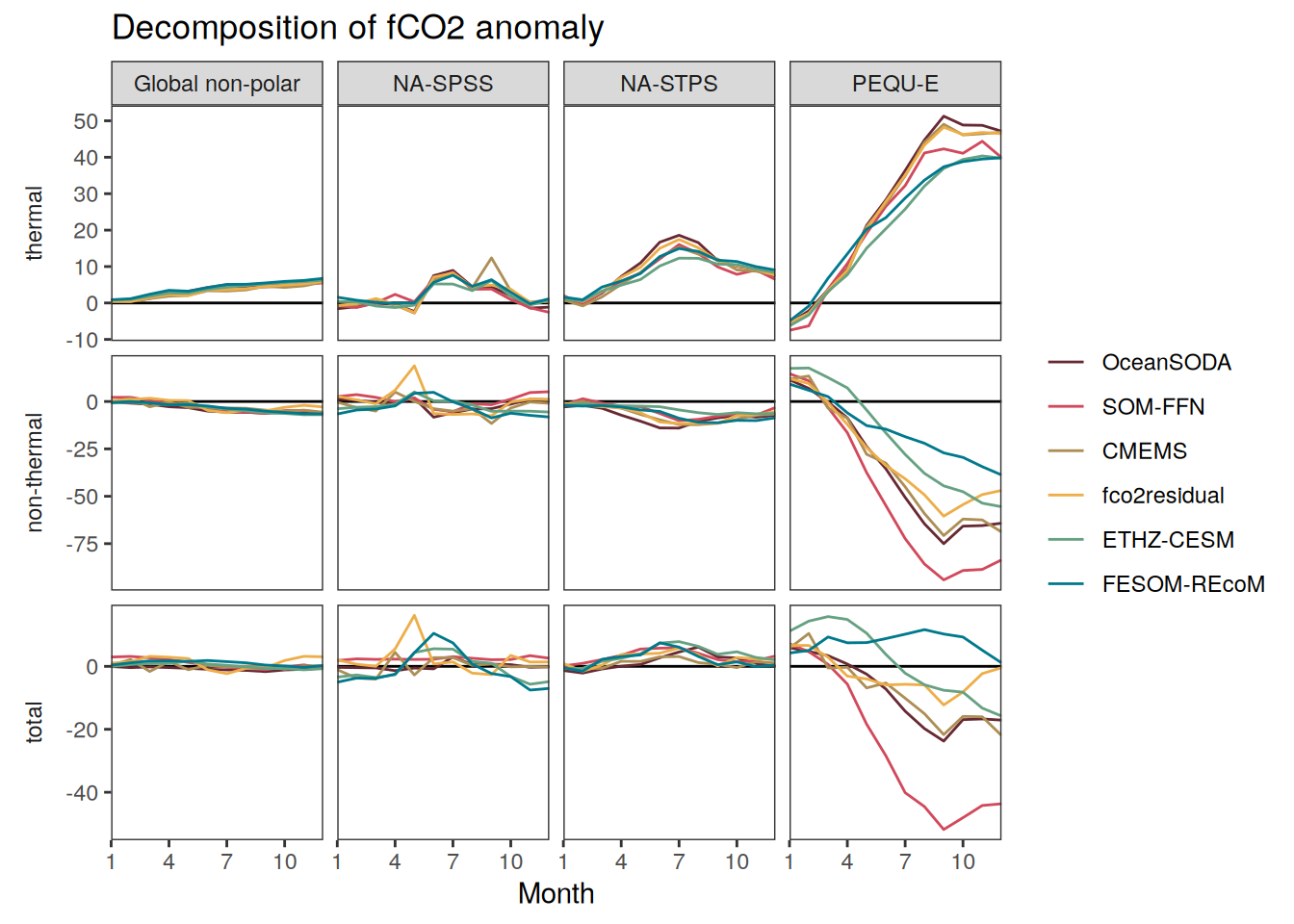
ggsave(width = 9,
       height = 4,
       dpi = 600,
       filename = "../output/biome_seasonal_anomaly_fco2_decomposition_all_products.pdf")
Biome profiles
The following analysis is available for GOBMs only.
Annual means
2023 anomaly
pco2_product_profiles_annual %>%
  filter(biome %in% key_biomes,
         name %in% name_core) %>%
  group_split(name) %>%
  # head(1) %>%
  map(
    ~ ggplot(data = .x) +
      geom_vline(xintercept = 0) +
      geom_path(aes(resid, depth, group = year), col = "grey30", alpha = 0.3) +
      geom_path(data = .x %>% filter(year == 2023),
                aes(resid, depth, col = as.factor(year)),
                linewidth = 1) +
      scale_color_brewer(palette = "Set1") +
      scale_y_continuous(trans = trans_reverser("sqrt"),
                         breaks = c(50,100,200,400)) +
      coord_cartesian(expand = 0) +
      facet_grid2(biome ~ product,
                  scales = "free_x", independent = "x") +
      labs(y = "Depth (m)",
           x = labels_breaks(.x %>% distinct(name))$i_legend_title) +
      theme(legend.title = element_blank(),
            axis.title.x = element_markdown())
  )
[[1]]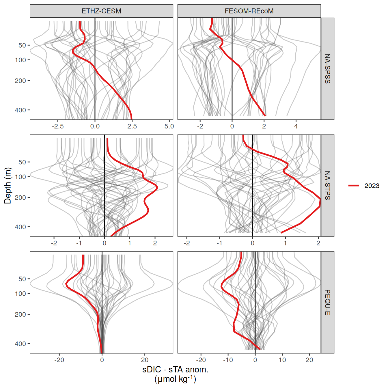
| Version | Author | Date |
|---|---|---|
| 518e3d0 | jens-daniel-mueller | 2025-02-27 |
[[2]]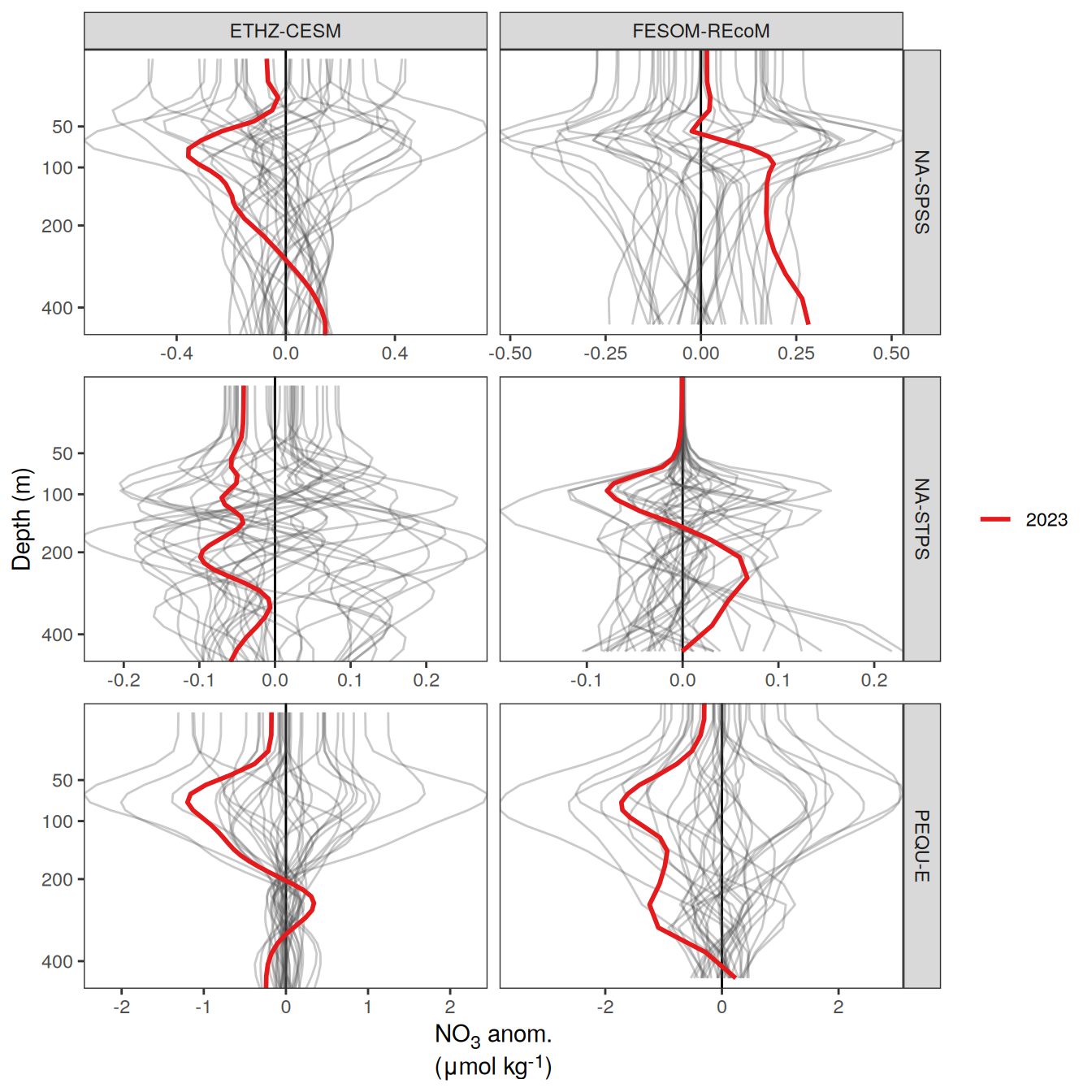
| Version | Author | Date |
|---|---|---|
| 518e3d0 | jens-daniel-mueller | 2025-02-27 |
[[3]]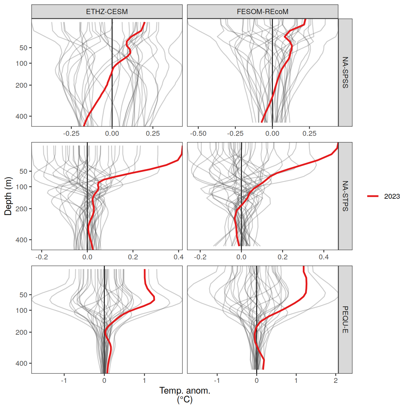
| Version | Author | Date |
|---|---|---|
| 518e3d0 | jens-daniel-mueller | 2025-02-27 |
Surface anomaly conversion
pco2_product_profiles_monthly_conversion <-
  read_csv(c("../data/ETHZ-CESM_2023_profiles_monthly.csv",
             "../data/FESOM-REcoM_2023_profiles_monthly.csv"),
           id = "product")

library(seacarb)

pco2_product_profiles_monthly_conversion <-
pco2_product_profiles_monthly_conversion %>%
  filter(biome %in% key_biomes,
         name %in% c("stalk", "sdissic", "thetao"),
         year == 2023,
         depth <= 5) %>%
  select(product, name, biome, month, value, resid) %>%
  group_by(name, biome, month) %>%
  summarise(value = mean(value),
            resid = mean(resid)) %>%
  ungroup() %>%
  pivot_wider(values_from = c(value, resid)) %>%
  mutate(buffesm(
    flag = 15,
    var1 = value_stalk * 1e-6,
    var2 = value_sdissic * 1e-6,
    T = value_thetao
  )[c(1, 4)],
  carb(
    flag = 15,
    var1 = value_stalk * 1e-6,
    var2 = value_sdissic * 1e-6,
    T = value_thetao
  )[c(8)]) %>%
  mutate(
    resid_fco2_stalk = gammaALK^-1 * fCO2 * resid_stalk * 1e-6,
    resid_fco2_sdissic = gammaALK^-1 * fCO2 * resid_sdissic * 1e-6,
    resid_fco2 = resid_fco2_stalk + resid_fco2_sdissic
  ) %>%
  select(biome, month, starts_with("resid")) %>%
  pivot_longer(starts_with("resid")) %>%
  arrange(month) %>%
  group_by(biome, name) %>%
  mutate(value = value - first(value)) %>%
  ungroup()


pco2_product_profiles_monthly_conversion %>%
  ggplot(aes(month, value)) +
  geom_hline(yintercept = 0) +
  geom_path() +
  facet_grid(biome ~ name, scales = "free_y")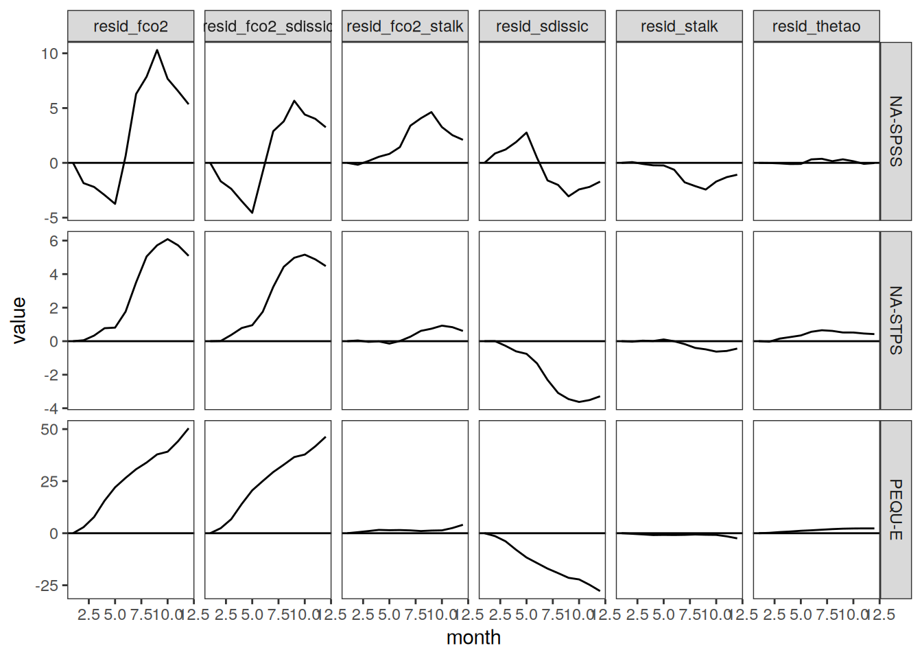
| Version | Author | Date |
|---|---|---|
| 3a5d484 | jens-daniel-mueller | 2025-03-11 |
pco2_product_profiles_monthly_conversion %>%
  filter(month == 12)
# A tibble: 18 × 4
biome month name value
<chr> <dbl> <chr> <dbl>
1 NA-SPSS 12 resid_sdissic -1.71
2 NA-SPSS 12 resid_stalk -1.08
3 NA-SPSS 12 resid_thetao -0.0169
4 NA-SPSS 12 resid_fco2_stalk 2.10
5 NA-SPSS 12 resid_fco2_sdissic 3.25
6 NA-SPSS 12 resid_fco2 5.35
7 NA-STPS 12 resid_sdissic -3.29
8 NA-STPS 12 resid_stalk -0.441
9 NA-STPS 12 resid_thetao 0.422
10 NA-STPS 12 resid_fco2_stalk 0.610
11 NA-STPS 12 resid_fco2_sdissic 4.48
12 NA-STPS 12 resid_fco2 5.09
13 PEQU-E 12 resid_sdissic -27.8
14 PEQU-E 12 resid_stalk -2.48
15 PEQU-E 12 resid_thetao 2.31
16 PEQU-E 12 resid_fco2_stalk 4.06
17 PEQU-E 12 resid_fco2_sdissic 46.3
18 PEQU-E 12 resid_fco2 50.4 Monthly means
2023 anomaly
pco2_product_profiles_monthly %>%
  filter(year == 2023,
         biome %in% key_biomes,
         name %in% name_core) %>%
  group_split(name) %>%
  # head(1) %>%
  map(
    ~ ggplot(data = .x) +
      geom_vline(xintercept = 0) +
      geom_path(aes(resid, depth, col = as.factor(month)),
                linewidth = 1) +
      scale_color_viridis_d(option = "magma", end = .8) +
      scale_y_continuous(trans = trans_reverser("sqrt"),
                         breaks = c(50,100,200,400)) +
      coord_cartesian(expand = 0) +
      facet_grid2(biome ~ product,
                  scales = "free_x", independent = "x") +
      labs(y = "Depth (m)",
           x = labels_breaks(.x %>% distinct(name))$i_legend_title) +
      theme(legend.title = element_blank(),
            axis.title.x = element_markdown())
  )
[[1]]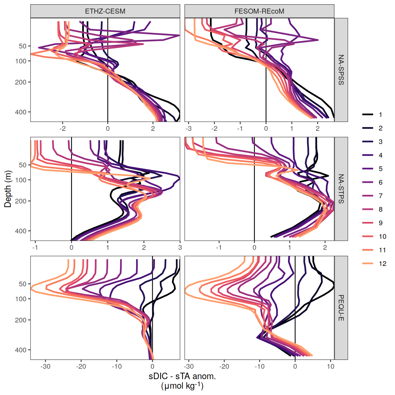
| Version | Author | Date |
|---|---|---|
| 518e3d0 | jens-daniel-mueller | 2025-02-27 |
[[2]]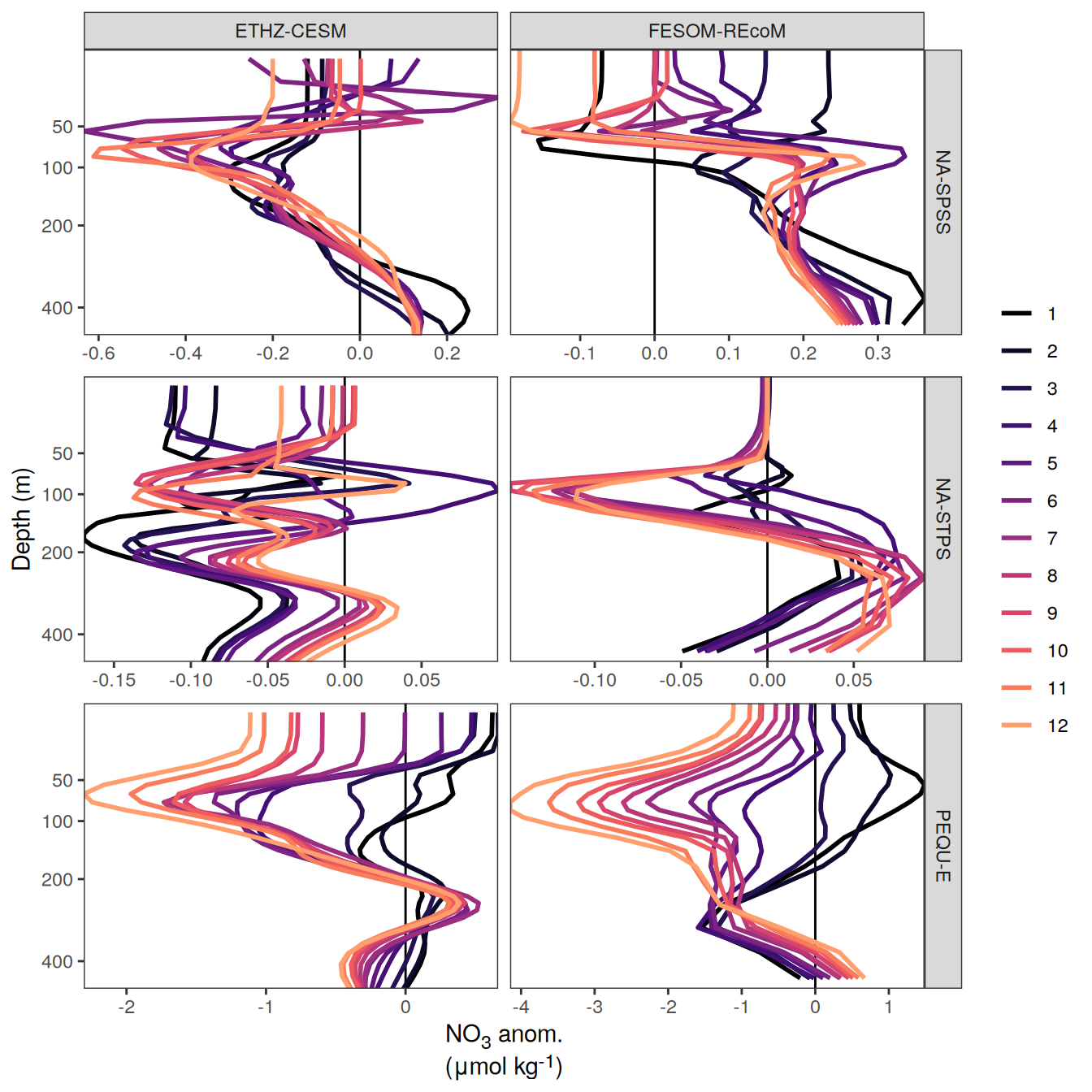
| Version | Author | Date |
|---|---|---|
| 518e3d0 | jens-daniel-mueller | 2025-02-27 |
[[3]]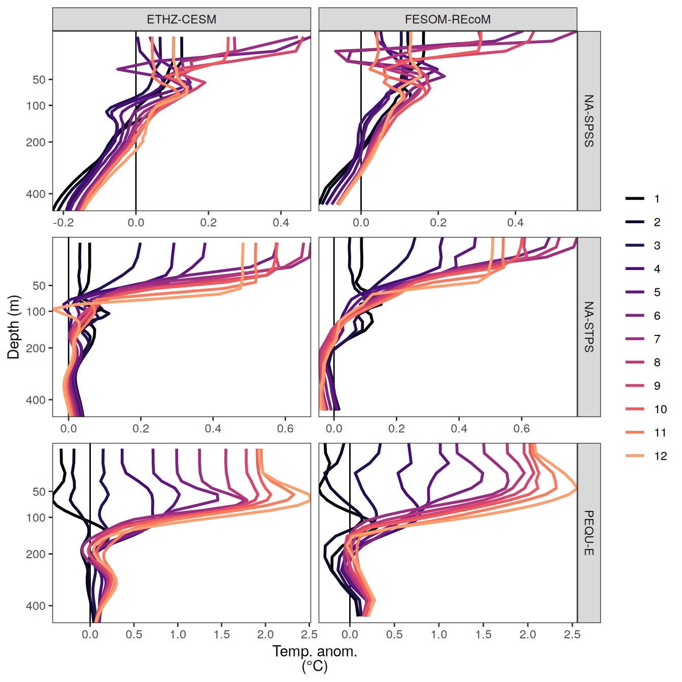
| Version | Author | Date |
|---|---|---|
| 518e3d0 | jens-daniel-mueller | 2025-02-27 |
pco2_product_profiles_monthly %>%
  filter(year == 2023,
         biome %in% key_biomes,
         product == "ETHZ-CESM",
         name %in% name_core) %>%
  ggplot() +
  geom_vline(xintercept = 0) +
  geom_path(aes(resid, depth, col = as.factor(month)),
            linewidth = 1) +
  scale_color_viridis_d(option = "magma", end = .8,
                        name = paste("Month of\n", 2023)) +
  scale_y_continuous(trans = trans_reverser("sqrt"),
                     breaks = c(50, 100, 200, 400)) +
  coord_cartesian(expand = 0) +
  facet_grid2(
    biome ~ name,
    scales = "free_x",
    independent = "x",
    labeller = labeller(name = x_axis_labels),
    switch = "x"
  ) +
  theme(
    strip.text.x.bottom = element_markdown(),
    strip.placement = "outside",
    strip.background.x = element_blank(),
    axis.title.x = element_blank()
  ) +
  labs(y = "Depth (m)",
       title = "Anomalies from monthly baseline (deseasonalized)")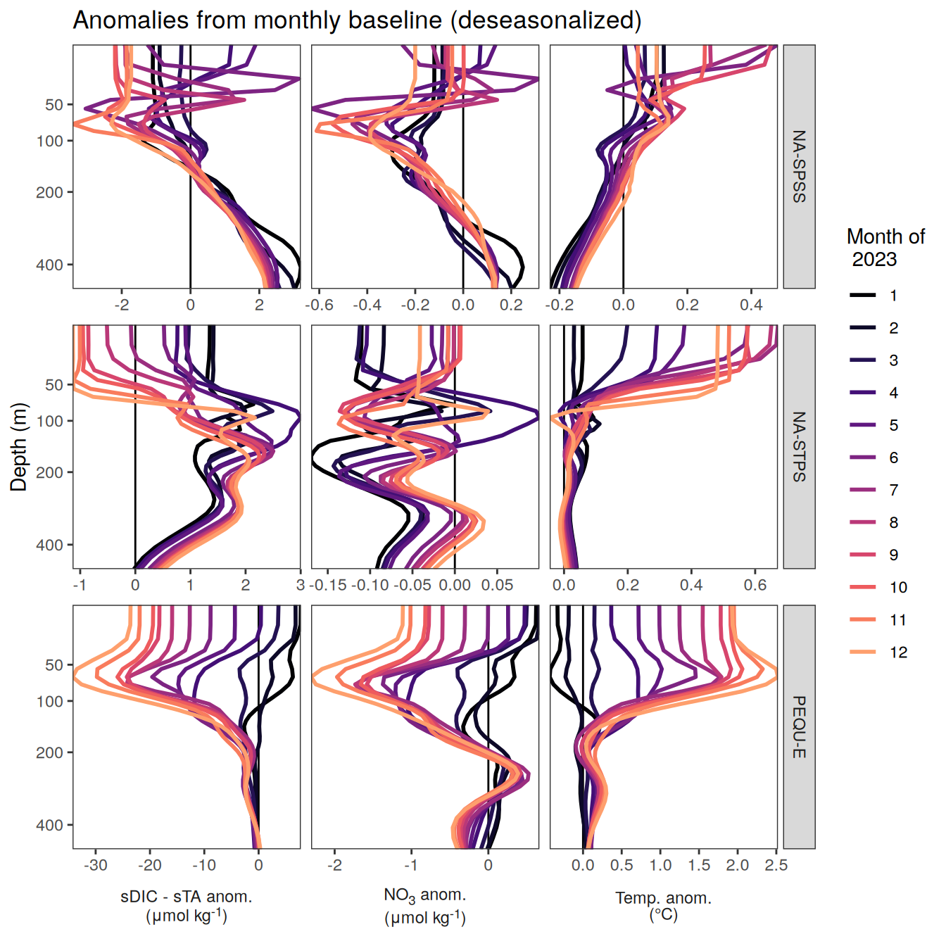
| Version | Author | Date |
|---|---|---|
| 518e3d0 | jens-daniel-mueller | 2025-02-27 |
# ggsave(width = 10,
#        height = 8,
#        dpi = 600,
#        filename = "../output/CESM_2023_anomaly_profiles.pdf")

pco2_product_profiles_monthly %>%
  filter(year == 2023,
         biome %in% key_biomes,
         product == "ETHZ-CESM",
         name %in% name_core) %>%
  arrange(month) %>%
  group_by(biome, name, depth) %>%
  mutate(resid = resid - first(resid)) %>%
  ungroup() %>%
  ggplot() +
  geom_vline(xintercept = 0) +
  geom_path(aes(resid, depth, col = as.factor(month)),
            linewidth = 1) +
  scale_color_viridis_d(option = "magma", end = .8,
                        name = paste("Month of\n", 2023)) +
  scale_y_continuous(trans = trans_reverser("sqrt"),
                     breaks = c(50, 100, 200, 400)) +
  coord_cartesian(expand = 0) +
  facet_grid2(
    biome ~ name,
    scales = "free_x",
    independent = "x",
    labeller = labeller(name = x_axis_labels),
    switch = "x"
  ) +
  theme(
    strip.text.x.bottom = element_markdown(),
    strip.placement = "outside",
    strip.background.x = element_blank(),
    axis.title.x = element_blank()
  ) +
  labs(y = "Depth (m)",
       title = "Monthly anomaly evolution relative to January 2023")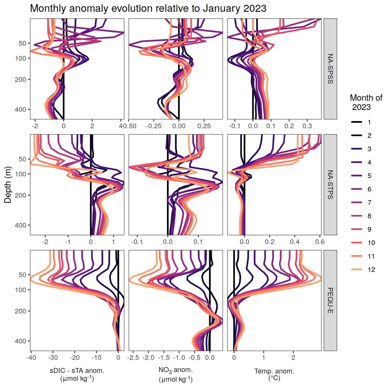
| Version | Author | Date |
|---|---|---|
| 518e3d0 | jens-daniel-mueller | 2025-02-27 |
pco2_product_profiles_monthly %>%
  filter(year == 2023,
         biome %in% key_biomes,
         product == "FESOM-REcoM",
         name %in% name_core) %>%
  ggplot() +
  geom_vline(xintercept = 0) +
  geom_path(aes(resid, depth, col = as.factor(month)),
            linewidth = 1) +
  scale_color_viridis_d(option = "magma", end = .8,
                        name = paste("Month of\n", 2023)) +
  scale_y_continuous(trans = trans_reverser("sqrt"),
                     breaks = c(50, 100, 200, 400)) +
  coord_cartesian(expand = 0) +
  facet_grid2(
    biome ~ name,
    scales = "free_x",
    independent = "x",
    labeller = labeller(name = x_axis_labels),
    switch = "x"
  ) +
  theme(
    strip.text.x.bottom = element_markdown(),
    strip.placement = "outside",
    strip.background.x = element_blank(),
    axis.title.x = element_blank()
  ) +
  labs(y = "Depth (m)",
       title = "Anomalies from monthly baseline (deseasonalized)")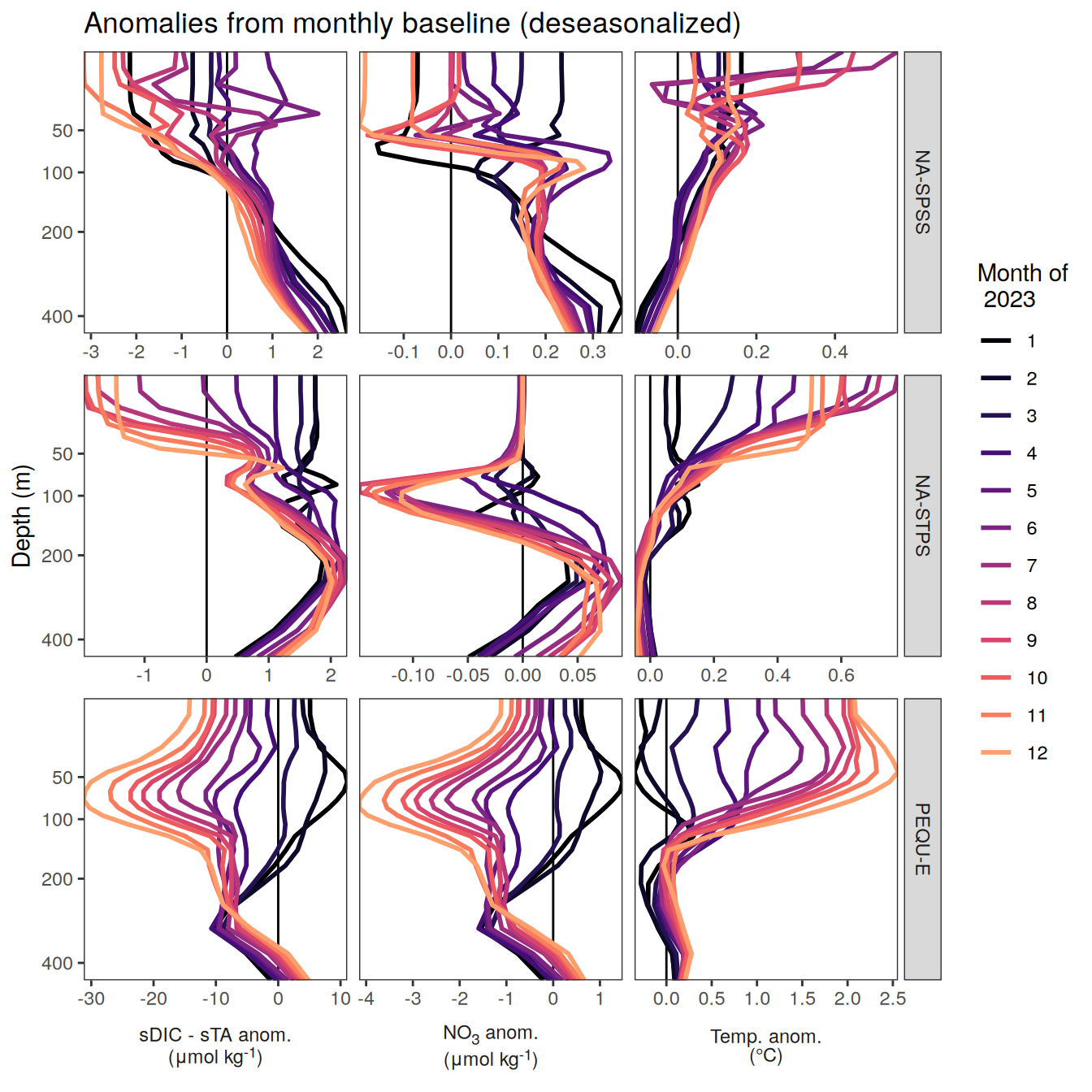
| Version | Author | Date |
|---|---|---|
| 518e3d0 | jens-daniel-mueller | 2025-02-27 |
# ggsave(width = 10,
#        height = 8,
#        dpi = 600,
#        filename = "../output/FESOM_2023_anomaly_profiles.pdf")
Hovmoeller
plot_list <-
  full_join(
    pco2_product_profiles_monthly %>%
      filter(
        year == 2023,
        biome %in% key_biomes,
        name %in% c("sdissic_stalk", "thetao")
      ),
    pco2_product_biome_monthly_detrended %>%
      filter(
        biome %in% key_biomes,
        name %in% "mld",
        year == 2023,
        product %in% gobm_product_list
      ) %>%
      select(product, month, biome, mld = value)
  ) %>%
  group_split(name, biome) %>%
  # head(1) %>%
  map(
    ~ ggplot(data = .x) +
      geom_contour_filled(aes(month, depth, z = resid)) +
      geom_line(aes(month, mld))+
      scale_fill_gradientn(
        colours = warm_cool_gradient,
        rescaler = ~ scales::rescale_mid(.x, mid = 0),
        super = ScaleDiscretised,
        name = labels_breaks(.x %>% distinct(name))$i_legend_title
      )+
      scale_y_continuous(trans = trans_reverser("sqrt"), breaks = c(20, 50, 100, 200, 400)) +
      coord_cartesian(expand = 0,
                      ylim = c(300,NA)) +
      facet_grid(product ~ biome) +
      guides(
        fill = guide_colorsteps(
          barheight = unit(0.3, "cm"),
          barwidth = unit(10, "cm"),
          ticks = TRUE,
          ticks.colour = "grey20",
          frame.colour = "grey20",
          label.position = "top",
          direction = "horizontal"
        )
      ) +
      theme(
        legend.position = "top",
        legend.title.align = 1,
        legend.box.spacing = unit(0.1, "cm"),
        legend.title = element_markdown(halign = 1,
                                        lineheight = 1.5)
      )
  )

plot_list
[[1]]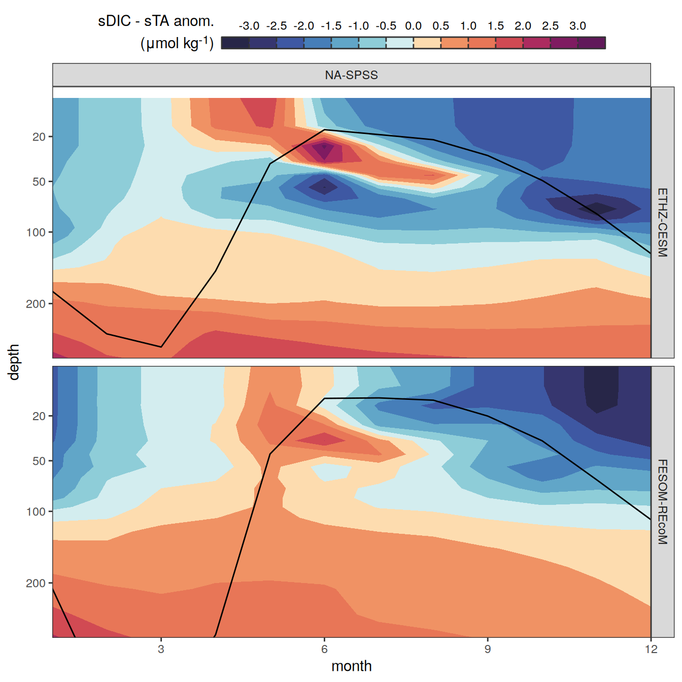
| Version | Author | Date |
|---|---|---|
| 518e3d0 | jens-daniel-mueller | 2025-02-27 |
[[2]]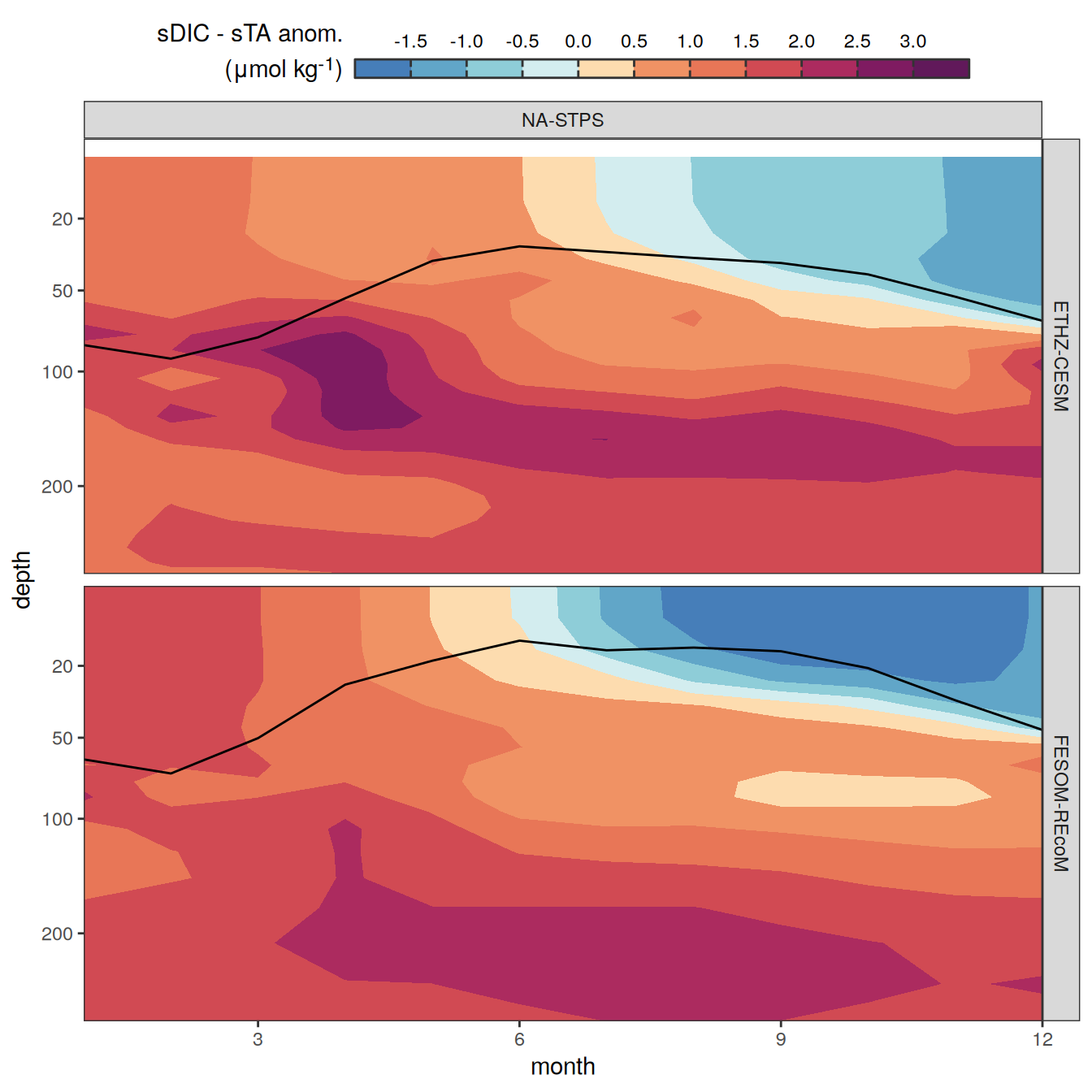
| Version | Author | Date |
|---|---|---|
| 518e3d0 | jens-daniel-mueller | 2025-02-27 |
[[3]]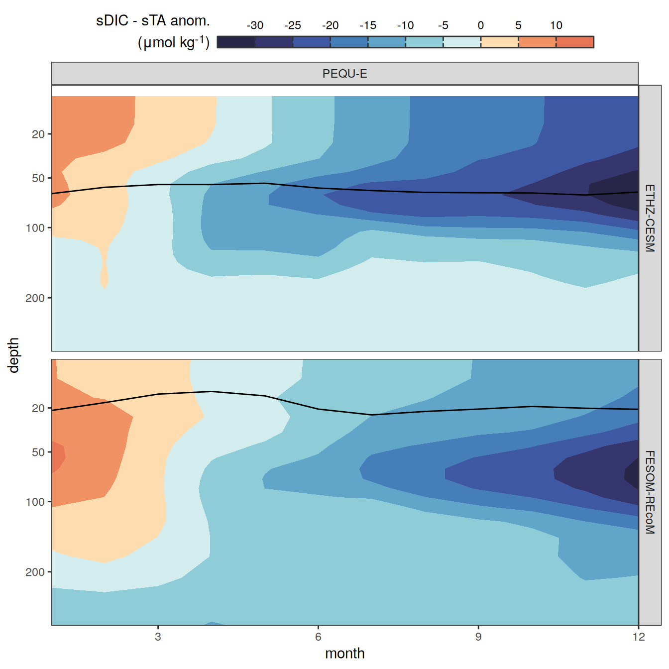
| Version | Author | Date |
|---|---|---|
| 518e3d0 | jens-daniel-mueller | 2025-02-27 |
[[4]]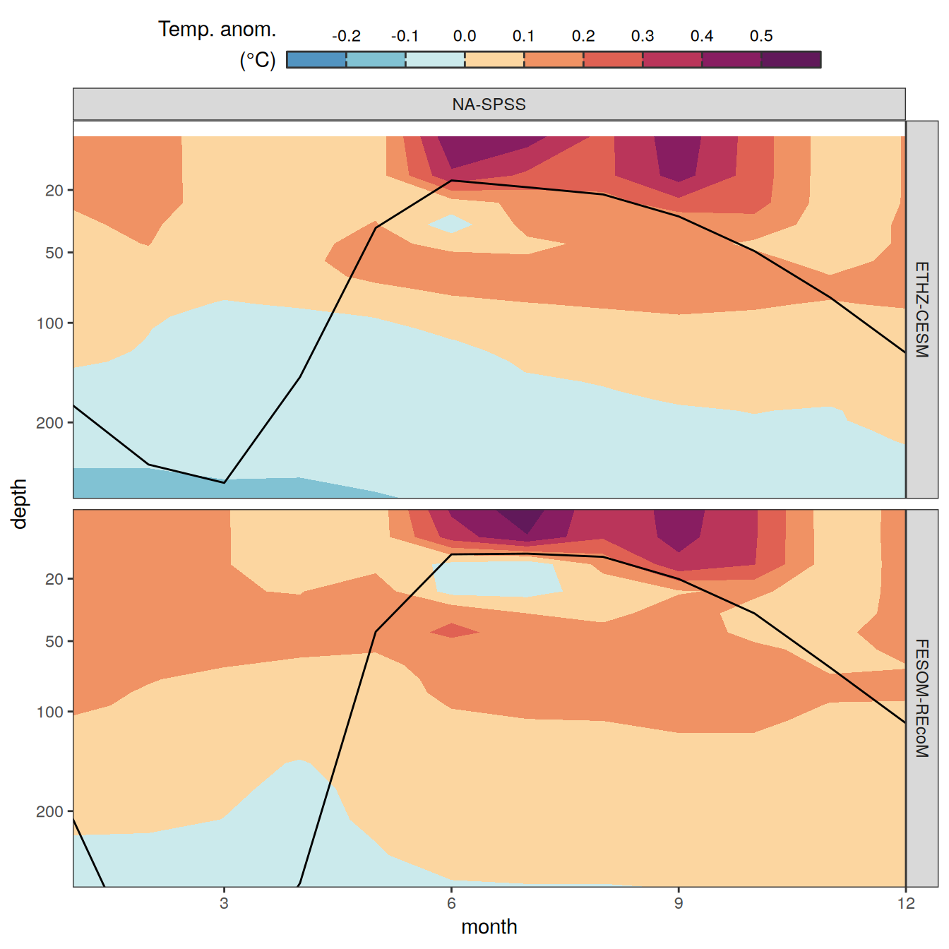
| Version | Author | Date |
|---|---|---|
| 518e3d0 | jens-daniel-mueller | 2025-02-27 |
[[5]]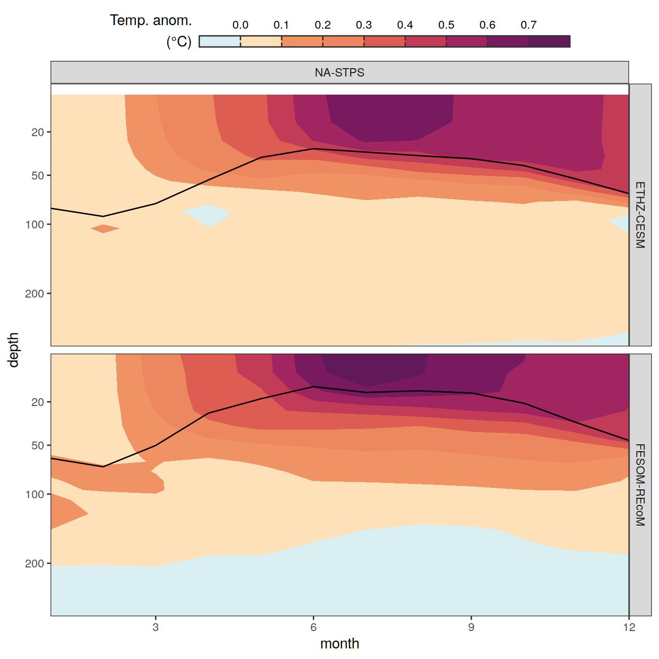
| Version | Author | Date |
|---|---|---|
| 518e3d0 | jens-daniel-mueller | 2025-02-27 |
[[6]]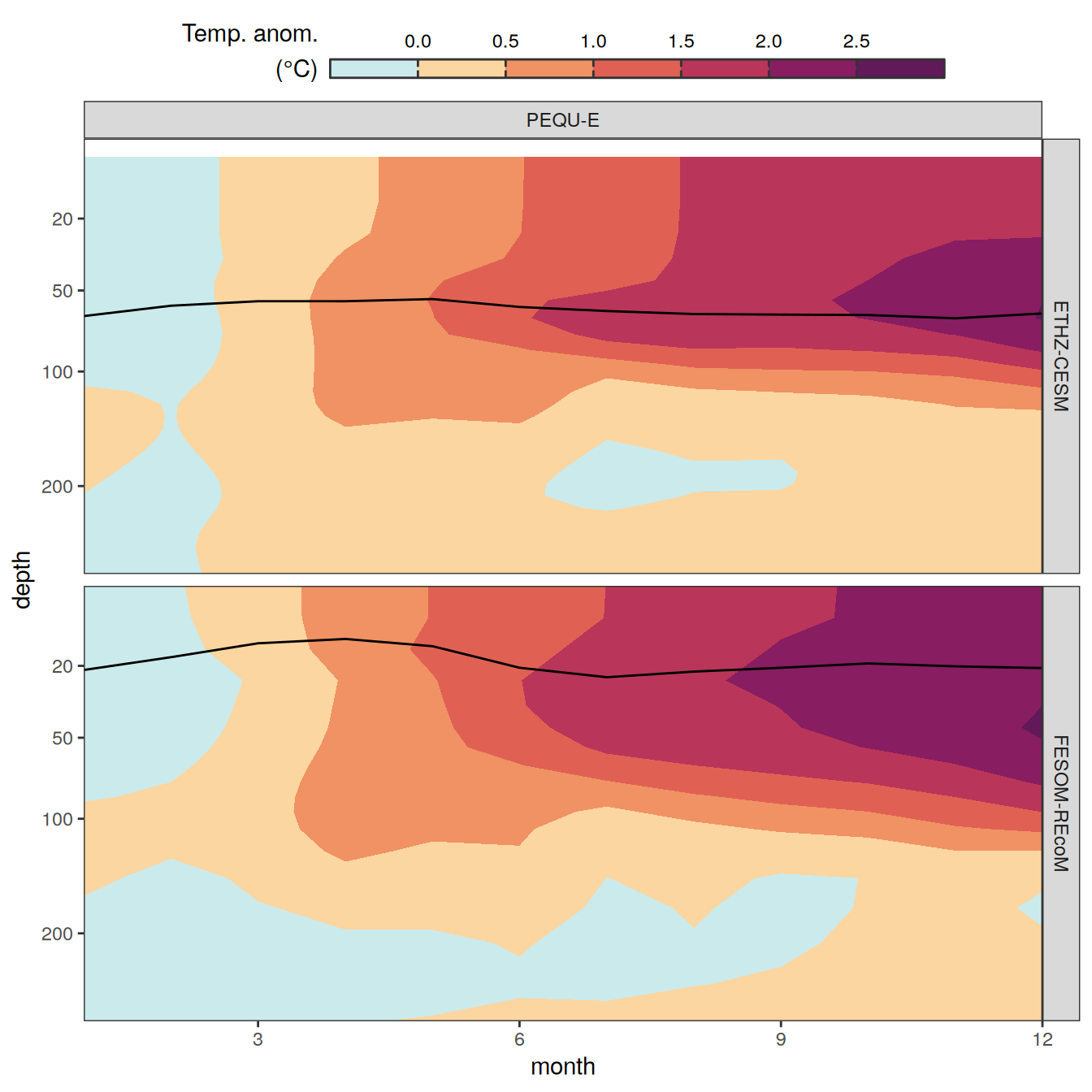
| Version | Author | Date |
|---|---|---|
| 518e3d0 | jens-daniel-mueller | 2025-02-27 |
ggsave(plot = wrap_plots(plot_list,
                         ncol = 3),
       width = 18,
       height = 12,
       dpi = 600,
       filename = "../output/profiles_hovmoeller_all_gobm.pdf")

plot_list <-
  full_join(
    pco2_product_profiles_monthly %>%
      filter(
        year == 2023,
        biome %in% key_biomes,
        name %in% c("sdissic_stalk", "thetao")
      ) %>%
      arrange(month) %>%
      group_by(product, name, biome, depth) %>%
      mutate(resid = if_else(name == "sdissic_stalk",
                             resid - first(resid),
                             resid)) %>%
      ungroup(),
    pco2_product_biome_monthly_detrended %>%
      filter(
        biome %in% key_biomes,
        name %in% "mld",
        year == 2023,
        product %in% gobm_product_list
      ) %>%
      select(product, month, biome, mld = value)
  ) %>%
  group_split(name, biome) %>%
  # head(1) %>%
  map(
    ~ ggplot(data = .x) +
      geom_contour_filled(aes(month, depth, z = resid)) +
      geom_line(aes(month, mld))+
      scale_fill_gradientn(
        colours = warm_cool_gradient,
        rescaler = ~ scales::rescale_mid(.x, mid = 0),
        super = ScaleDiscretised,
        name = labels_breaks(.x %>% distinct(name))$i_legend_title
      )+
      scale_y_continuous(trans = trans_reverser("sqrt"), breaks = c(20, 50, 100, 200, 400)) +
      coord_cartesian(expand = 0,
                      ylim = c(300,NA)) +
      facet_grid(product ~ biome) +
      guides(
        fill = guide_colorsteps(
          barheight = unit(0.3, "cm"),
          barwidth = unit(10, "cm"),
          ticks = TRUE,
          ticks.colour = "grey20",
          frame.colour = "grey20",
          label.position = "top",
          direction = "horizontal"
        )
      ) +
      theme(
        legend.position = "top",
        legend.title.align = 1,
        legend.box.spacing = unit(0.1, "cm"),
        legend.title = element_markdown(halign = 1,
                                        lineheight = 1.5)
      )
  )

ggsave(plot = wrap_plots(plot_list,
                         ncol = 3),
       width = 18,
       height = 12,
       dpi = 600,
       filename = "../output/profiles_hovmoeller_all_gobm_evolution.pdf")
CESM_depth_grid <- pco2_product_profiles_monthly %>%
filter(year == 2023,
product == "ETHZ-CESM",
biome %in% key_biomes,
name %in% c("sdissic_stalk", "thetao")) %>%
distinct(name, biome, month, depth)
pco2_product_profiles_monthly_FESOM_regrid <-
full_join(
pco2_product_profiles_monthly %>%
filter(
year == 2023,
product == "FESOM-REcoM",
biome %in% key_biomes,
name %in% c("sdissic_stalk", "thetao")
),
CESM_depth_grid %>% mutate(product = "FESOM-REcoM")
)
pco2_product_profiles_monthly_FESOM_regrid <-
pco2_product_profiles_monthly_FESOM_regrid %>%
arrange(product, name, biome, month, depth)
pco2_product_profiles_monthly_FESOM_regrid <-
pco2_product_profiles_monthly_FESOM_regrid %>%
arrange(depth) %>%
group_by(product, name, biome, month) %>%
mutate(resid = spline(
depth,
resid,
method = "natural",
xout = depth
)$y) %>%
ungroup()
CESM_depth <-
CESM_depth_grid %>% distinct(depth) %>% pull()
pco2_product_profiles_monthly_FESOM_regrid <-
pco2_product_profiles_monthly_FESOM_regrid %>%
filter(depth %in% CESM_depth)
pco2_product_profiles_monthly_merged <-
bind_rows(
pco2_product_profiles_monthly_FESOM_regrid,
pco2_product_profiles_monthly %>%
filter(
year == 2023,
product == "ETHZ-CESM",
biome %in% key_biomes,
name %in% c("sdissic_stalk", "thetao")
)
)
pco2_product_profiles_monthly_ensemble <-
pco2_product_profiles_monthly_merged %>%
group_by(name, biome, month, depth) %>%
summarise(resid = mean(resid)) %>%
ungroup()
pco2_product_profiles_monthly_ensemble <-
full_join(
pco2_product_profiles_monthly_ensemble %>%
filter(
biome %in% key_biomes,
name %in% c("sdissic_stalk", "thetao")
),
pco2_product_biome_monthly_detrended %>%
filter(
biome %in% key_biomes,
name %in% "mld",
year == 2023,
product %in% gobm_product_list
) %>%
group_by(month, biome) %>%
summarise(mld = mean(value)) %>%
ungroup()
)
# plot_list <-
pco2_product_profiles_monthly_ensemble %>%
group_split(name, biome) %>%
head(1) %>%
map(
~ ggplot(data = .x) +
geom_contour_filled(aes(month, depth, z = resid)) +
geom_line(aes(month, mld)) +
scale_fill_gradientn(
colours = warm_cool_gradient,
rescaler = ~ scales::rescale_mid(.x, mid = 0),
super = ScaleDiscretised,
name = labels_breaks(.x %>% distinct(name))$i_legend_title
) +
scale_y_continuous(trans = trans_reverser("sqrt"), breaks = c(50, 100, 200, 400)) +
coord_cartesian(expand = 0, ylim = c(300, NA)) +
facet_wrap(~ biome) +
guides(
fill = guide_colorsteps(
barheight = unit(0.3, "cm"),
barwidth = unit(10, "cm"),
ticks = TRUE,
ticks.colour = "grey20",
frame.colour = "grey20",
label.position = "top",
direction = "horizontal"
)
) +
theme(
legend.position = "top",
legend.title.align = 1,
legend.box.spacing = unit(0.1, "cm"),
legend.title = element_markdown(halign = 1, lineheight = 1.5)
)
)[[1]]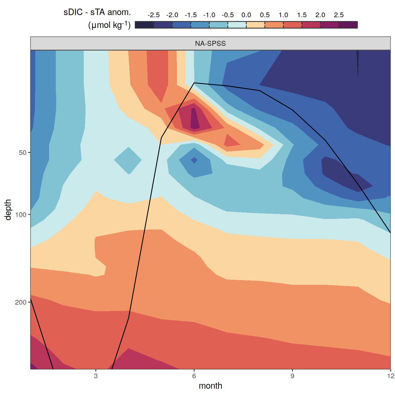
| Version | Author | Date |
|---|---|---|
| 518e3d0 | jens-daniel-mueller | 2025-02-27 |
ggsave(plot = wrap_plots(plot_list,
                         ncol = 3),
       width = 18,
       height = 8,
       dpi = 600,
       filename = "../output/profiles_hovmoeller_ensemble_mean_gobm.pdf")
labels_breaks_hov <- function(i_name, i_biome) {
if (i_name == "sdissic_stalk") {
i_legend_title <- "sDIC - sTA<br>anom.<br>(μmol kg<sup>-1</sup>)"
}
if (i_name == "thetao") {
i_legend_title <- "Temp.<br>anom.<br>(°C)"
}
if (i_name == "sdissic_stalk" & i_biome == "NA-SPSS") {
i_breaks <- c(-Inf, seq(-2, 2, 0.5), Inf)
}
if (i_name == "thetao" & i_biome == "NA-SPSS") {
i_breaks <- c(-Inf, seq(-0.4, 0.4, 0.1), Inf)
}
if (i_name == "sdissic_stalk" & i_biome == "NA-STPS") {
i_breaks <- c(-Inf, seq(-2.4, 2.4, 0.6), Inf)
}
if (i_name == "thetao" & i_biome == "NA-STPS") {
i_breaks <- c(-Inf, seq(-0.6, 0.6, 0.15), Inf)
}
if (i_name == "sdissic_stalk" & i_biome == "PEQU-E") {
i_breaks <- c(-Inf, seq(-32, 32, 8), Inf)
}
if (i_name == "thetao" & i_biome == "PEQU-E") {
i_breaks <- c(-Inf, seq(-2, 2, 0.5), Inf)
}
i_breaks_labels <- i_breaks[!i_breaks == Inf]
i_breaks_labels <- i_breaks_labels[!i_breaks_labels == -Inf]
i_breaks_labels[seq_along(i_breaks_labels) %% 2 == 0] <- ""
all_labels_breaks <- lst(i_legend_title, i_breaks, i_breaks_labels)
return(all_labels_breaks)
}
labels_breaks_hov("sdissic_stalk", "NA-SPSS")$i_legend_title
[1] "sDIC - sTA<br>anom.<br>(μmol kg<sup>-1</sup>)"
$i_breaks
[1] -Inf -2.0 -1.5 -1.0 -0.5 0.0 0.5 1.0 1.5 2.0 Inf
$i_breaks_labels
[1] "-2" "" "-1" "" "0" "" "1" "" "2" plot_list_left <-
pco2_product_profiles_monthly_ensemble %>%
arrange(month) %>%
group_by(name, biome, depth) %>%
mutate(resid = if_else(name == "sdissic_stalk", resid - first(resid), resid)) %>%
ungroup() %>%
group_split(biome, name) %>%
head(2) %>%
map(
~ ggplot(data = .x) +
geom_contour_filled(aes(month, depth, z = resid),
breaks = labels_breaks_hov(.x %>% distinct(name),
.x %>% distinct(biome))$i_breaks) +
geom_line(aes(month, mld)) +
scale_fill_gradientn(
colours = warm_cool_gradient,
super = ScaleDiscretised,
name = labels_breaks_hov(.x %>% distinct(name),
.x %>% distinct(biome))$i_legend_title,
labels = labels_breaks_hov(.x %>% distinct(name),
.x %>% distinct(biome))$i_breaks_labels
) +
# scale_fill_gradientn(
# colours = warm_cool_gradient,
# rescaler = ~ scales::rescale_mid(.x, mid = 0),
# super = ScaleDiscretised,
# name = labels_breaks(.x %>% distinct(name))$i_legend_title
# ) +
scale_y_continuous(
trans = trans_reverser("sqrt"),
breaks = c(20, 50, 100, 200, 400)
) +
coord_cartesian(expand = 0, ylim = c(300, NA)) +
labs(y = "Depth (m)",
x = "Month") +
facet_wrap(~ biome) +
guides(
fill = guide_colorsteps(
barheight = unit(0.3, "cm"),
barwidth = unit(5, "cm"),
ticks = TRUE,
ticks.colour = "grey20",
frame.colour = "grey20",
label.position = "top",
direction = "horizontal"
)
) +
theme(
legend.position = "top",
legend.box.spacing = unit(0.1, "cm"),
legend.title = element_markdown(hjust = 1,
lineheight = 1.5)
)
)
plot_list_right <-
pco2_product_profiles_monthly_ensemble %>%
arrange(month) %>%
group_by(name, biome, depth) %>%
mutate(resid = if_else(name == "sdissic_stalk", resid - first(resid), resid)) %>%
ungroup() %>%
group_split(biome, name) %>%
tail(4) %>%
map(
~ ggplot(data = .x) +
geom_contour_filled(aes(month, depth, z = resid),
breaks = labels_breaks_hov(.x %>% distinct(name),
.x %>% distinct(biome))$i_breaks) +
geom_line(aes(month, mld)) +
scale_fill_gradientn(
colours = warm_cool_gradient,
super = ScaleDiscretised,
name = labels_breaks_hov(.x %>% distinct(name),
.x %>% distinct(biome))$i_legend_title,
labels = labels_breaks_hov(.x %>% distinct(name),
.x %>% distinct(biome))$i_breaks_labels
) +
scale_y_continuous(
trans = trans_reverser("sqrt"),
breaks = c(20, 50, 100, 200, 400)
) +
coord_cartesian(expand = 0, ylim = c(300, NA)) +
labs(y = "Depth (m)", x = "Month")+
facet_wrap(~ biome) +
guides(
fill = guide_colorsteps(
barheight = unit(0.3, "cm"),
barwidth = unit(5, "cm"),
ticks = TRUE,
ticks.colour = "grey20",
frame.colour = "grey20",
label.position = "top",
direction = "horizontal"
)
) +
theme(
legend.position = "top",
# legend.margin = margin(0, 0, 0, 0),
# legend.justification = "left",
axis.title.y = element_blank(),
axis.text.y = element_blank(),
legend.title.align = 1,
legend.box.spacing = unit(0.1, "cm"),
legend.title = element_blank()
)
)
plot_list <- c(plot_list_left, plot_list_right)
ggsave(plot = wrap_plots(plot_list,
ncol = 3,
byrow = FALSE),
width = 10,
height = 6,
dpi = 600,
filename = "../output/Fig4_cd.pdf")
plot_list_left <-
pco2_product_profiles_monthly_ensemble %>%
filter(biome == "NA-STPS") %>%
arrange(month) %>%
group_by(name, biome, depth) %>%
mutate(resid = if_else(name == "sdissic_stalk", resid - first(resid), resid)) %>%
ungroup() %>%
group_split(biome, name) %>%
map(
~ ggplot(data = .x) +
geom_contour_filled(aes(month, depth, z = resid),
breaks = labels_breaks_hov(.x %>% distinct(name),
.x %>% distinct(biome))$i_breaks) +
geom_line(aes(month, mld)) +
scale_fill_gradientn(
colours = warm_cool_gradient,
super = ScaleDiscretised,
name = labels_breaks_hov(.x %>% distinct(name),
.x %>% distinct(biome))$i_legend_title,
labels = labels_breaks_hov(.x %>% distinct(name),
.x %>% distinct(biome))$i_breaks_labels
) +
# scale_fill_gradientn(
# colours = warm_cool_gradient,
# rescaler = ~ scales::rescale_mid(.x, mid = 0),
# super = ScaleDiscretised,
# name = labels_breaks(.x %>% distinct(name))$i_legend_title
# ) +
scale_y_continuous(
trans = trans_reverser("sqrt"),
breaks = c(20, 50, 100, 200, 400)
) +
coord_cartesian(expand = 0, ylim = c(300, NA)) +
labs(y = "Depth (m)",
x = "Month") +
facet_wrap(~ biome) +
guides(
fill = guide_colorsteps(
barheight = unit(0.3, "cm"),
barwidth = unit(5, "cm"),
ticks = TRUE,
ticks.colour = "grey20",
frame.colour = "grey20",
label.position = "top",
direction = "horizontal"
)
) +
theme(
legend.position = "top",
legend.box.spacing = unit(0.1, "cm"),
legend.title = element_markdown(hjust = 1,
lineheight = 1.5)
)
)
plot_list_right <-
pco2_product_profiles_monthly_ensemble %>%
filter(biome == "PEQU-E") %>%
arrange(month) %>%
group_by(name, biome, depth) %>%
mutate(resid = if_else(name == "sdissic_stalk", resid - first(resid), resid)) %>%
ungroup() %>%
group_split(biome, name) %>%
# tail(4) %>%
map(
~ ggplot(data = .x) +
geom_contour_filled(aes(month, depth, z = resid),
breaks = labels_breaks_hov(.x %>% distinct(name),
.x %>% distinct(biome))$i_breaks) +
geom_line(aes(month, mld)) +
scale_fill_gradientn(
colours = warm_cool_gradient,
super = ScaleDiscretised,
name = labels_breaks_hov(.x %>% distinct(name),
.x %>% distinct(biome))$i_legend_title,
labels = labels_breaks_hov(.x %>% distinct(name),
.x %>% distinct(biome))$i_breaks_labels
) +
scale_y_continuous(
trans = trans_reverser("sqrt"),
breaks = c(20, 50, 100, 200, 400)
) +
coord_cartesian(expand = 0, ylim = c(300, NA)) +
labs(y = "Depth (m)", x = "Month")+
facet_wrap(~ biome) +
guides(
fill = guide_colorsteps(
barheight = unit(0.3, "cm"),
barwidth = unit(5, "cm"),
ticks = TRUE,
ticks.colour = "grey20",
frame.colour = "grey20",
label.position = "top",
direction = "horizontal"
)
) +
theme(
legend.position = "top",
# legend.margin = margin(0, 0, 0, 0),
# legend.justification = "left",
axis.title.y = element_blank(),
axis.text.y = element_blank(),
legend.title.align = 1,
legend.box.spacing = unit(0.1, "cm"),
legend.title = element_blank()
)
)
plot_list <- c(plot_list_left, plot_list_right)
ggsave(plot = wrap_plots(plot_list,
ncol = 2,
byrow = FALSE),
width = 7,
height = 6,
dpi = 1200,
filename = "../output/profiles_hovmoeller_ensemble_mean_gobm_evolution_2_biomes.pdf")
sessionInfo()R version 4.4.2 (2024-10-31)
Platform: x86_64-pc-linux-gnu
Running under: openSUSE Leap 15.6
Matrix products: default
BLAS/LAPACK: /usr/local/OpenBLAS-0.3.28/lib/libopenblas_haswellp-r0.3.28.so; LAPACK version 3.12.0
locale:
[1] LC_CTYPE=en_US.UTF-8 LC_NUMERIC=C
[3] LC_TIME=en_US.UTF-8 LC_COLLATE=en_US.UTF-8
[5] LC_MONETARY=en_US.UTF-8 LC_MESSAGES=en_US.UTF-8
[7] LC_PAPER=en_US.UTF-8 LC_NAME=C
[9] LC_ADDRESS=C LC_TELEPHONE=C
[11] LC_MEASUREMENT=en_US.UTF-8 LC_IDENTIFICATION=C
time zone: Europe/Zurich
tzcode source: system (glibc)
attached base packages:
[1] stats graphics grDevices utils datasets methods base
other attached packages:
[1] seacarb_3.3.3 SolveSAPHE_2.1.0 oce_1.8-3
[4] gsw_1.2-0 kableExtra_1.4.0 cmocean_0.3-2
[7] ggh4x_0.3.0 scales_1.3.0 biscale_1.0.0
[10] ggtext_0.1.2 khroma_1.14.0 ggnewscale_0.5.0
[13] terra_1.8-5 sf_1.0-19 rnaturalearth_1.0.1
[16] geomtextpath_0.1.4 colorspace_2.1-1 marelac_2.1.11
[19] shape_1.4.6.1 ggforce_0.4.2 metR_0.16.0
[22] scico_1.5.0 patchwork_1.3.0 collapse_2.0.18
[25] lubridate_1.9.3 forcats_1.0.0 stringr_1.5.1
[28] dplyr_1.1.4 purrr_1.0.2 readr_2.1.5
[31] tidyr_1.3.1 tibble_3.2.1 ggplot2_3.5.1
[34] tidyverse_2.0.0
loaded via a namespace (and not attached):
[1] DBI_1.2.3 rlang_1.1.4 magrittr_2.0.3
[4] git2r_0.35.0 e1071_1.7-16 compiler_4.4.2
[7] mgcv_1.9-1 systemfonts_1.1.0 vctrs_0.6.5
[10] pkgconfig_2.0.3 crayon_1.5.3 fastmap_1.2.0
[13] backports_1.5.0 labeling_0.4.3 utf8_1.2.4
[16] promises_1.3.2 rmarkdown_2.29 markdown_1.13
[19] tzdb_0.4.0 ragg_1.3.3 bit_4.5.0
[22] xfun_0.49 cachem_1.1.0 jsonlite_1.8.9
[25] later_1.4.1 tweenr_2.0.3 parallel_4.4.2
[28] R6_2.5.1 RColorBrewer_1.1-3 bslib_0.8.0
[31] stringi_1.8.4 jquerylib_0.1.4 Rcpp_1.0.13-1
[34] knitr_1.49 Matrix_1.7-1 splines_4.4.2
[37] httpuv_1.6.15 timechange_0.3.0 tidyselect_1.2.1
[40] rstudioapi_0.17.1 yaml_2.3.10 codetools_0.2-20
[43] lattice_0.22-6 withr_3.0.2 evaluate_1.0.1
[46] isoband_0.2.7 rnaturalearthdata_1.0.0 units_0.8-5
[49] proxy_0.4-27 polyclip_1.10-7 xml2_1.3.6
[52] pillar_1.9.0 whisker_0.4.1 KernSmooth_2.23-24
[55] checkmate_2.3.2 generics_0.1.3 vroom_1.6.5
[58] rprojroot_2.0.4 hms_1.1.3 commonmark_1.9.2
[61] munsell_0.5.1 class_7.3-22 glue_1.8.0
[64] tools_4.4.2 data.table_1.16.2 fs_1.6.5
[67] cowplot_1.1.3 grid_4.4.2 nlme_3.1-166
[70] cli_3.6.3 textshaping_0.4.0 workflowr_1.7.1
[73] fansi_1.0.6 viridisLite_0.4.2 svglite_2.1.3
[76] gtable_0.3.6 sass_0.4.9 digest_0.6.37
[79] classInt_0.4-10 farver_2.1.2 memoise_2.0.1
[82] htmltools_0.5.8.1 lifecycle_1.0.4 httr_1.4.7
[85] here_1.0.1 gridtext_0.1.5 bit64_4.5.2
[88] MASS_7.3-61